Part 1: Finite Difference Operator and Derivative of Gaussian Filters
This section shows the results of applying the finite difference operator and derivative of Gaussian (DoG) filters to detect edges in the cameraman image.
Part 1.1: Finite Difference Operator
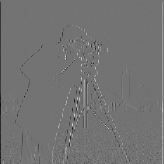
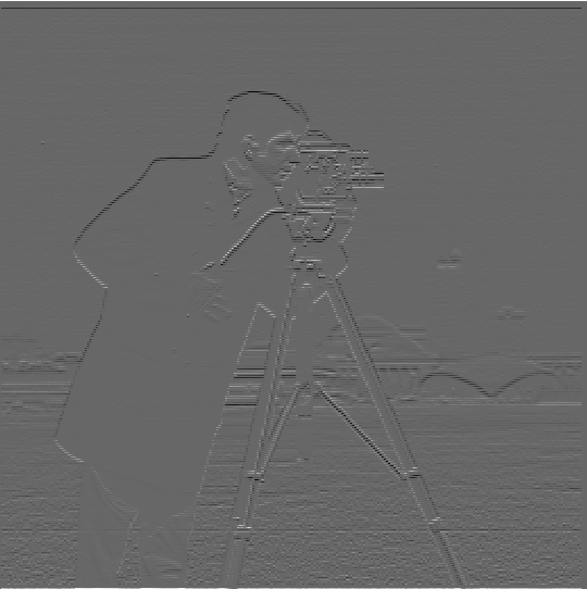
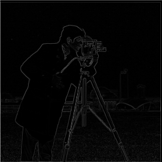
In this part, we convolve the image with finite difference operators in the X and Y directions to compute the partial derivatives and gradient magnitude. Gradient magnitude computation involves calculating the rate of intensity change at each pixel using the Euclidean norm of the partial derivatives in the 𝑥 and 𝑦 directions. This is done by convolving the image with finite difference kernels to obtain the derivatives, then combining them to compute the gradient magnitude. A threshold can be applied to highlight edges. Below are the results:
Edge Thresholding
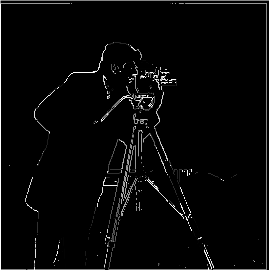
After calculating the gradient magnitude, we applied a threshold to create a binary edge image. Below is the thresholded edge image:
Part 1.2: Derivative of Gaussian (DoG) Filter
Part 1.2a: Smoothing Followed by Differentiating
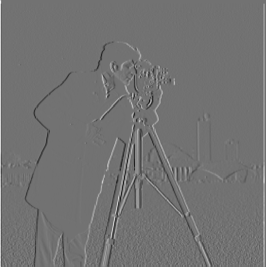
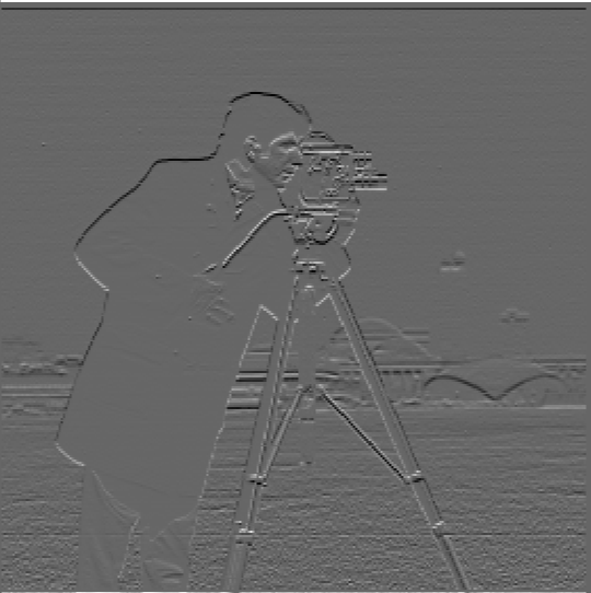
In this part, we applied a Gaussian filter to smooth the image first, and then computed the partial derivatives in X and Y directions. Below are the results after smoothing and differentiating:

Part 1.2b: Derivative of Gaussian (DoG) Filter
Next, we used the DoG filter, which combines smoothing and differentiation in a single step. Below are the results using the DoG filter:
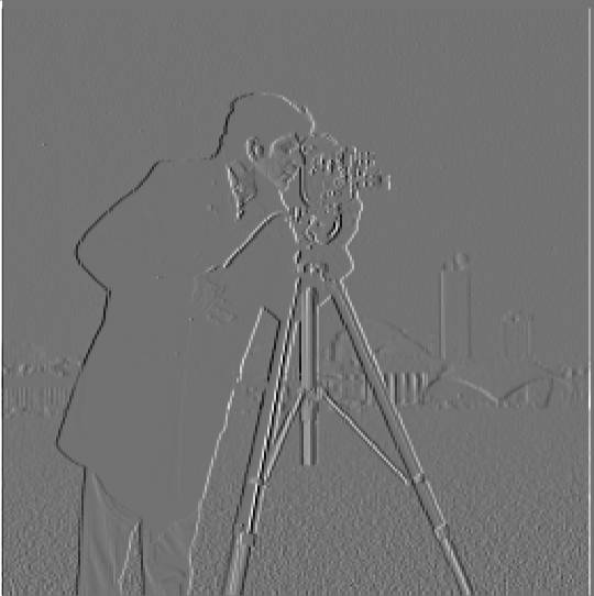
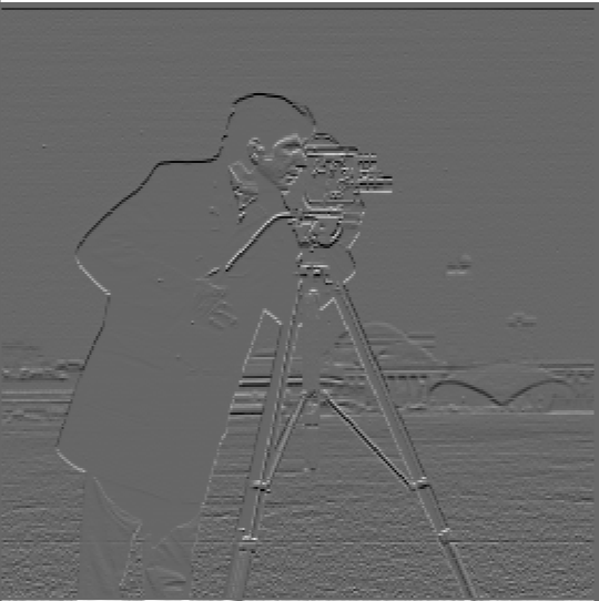
What differences do you see? When Gaussian smoothing is applied before differentiating, the resulting edges are smoother and less noisy compared to Part 1.1, which directly applies the finite difference operator. The smoothing step in this part reduces sensitivity to minor intensity variations, highlighting more meaningful edges while suppressing noise. In contrast, Part 1.1 produces noisier results, making it harder to isolate clear edges.
Verification: Comparison of Results
To verify that the DoG filter produces the same result as smoothing first and then differentiating, we compare the images generated by both methods. As shown below, the images for the X and Y partial derivatives using the two methods are nearly identical:


Part 2.1: Unsharp Masking
In this section, we use the unsharp masking technique to enhance the sharpness of a blurry image by adding back the high-frequency components. We first demonstrate the sharpening on a selected blurry image and then on a few example images.
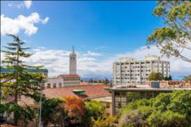
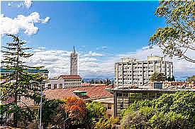
Blurry Image to Sharpened
This image was initially blurry, but after applying the unsharp masking filter, the image looks sharper and more detailed.
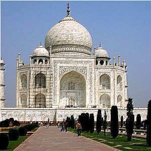
Taj Mahal: Original, Blurred, and Sharpened
Below are the three phases of processing the image: the original image, a blurred version, and the final sharpened version after applying unsharp masking.


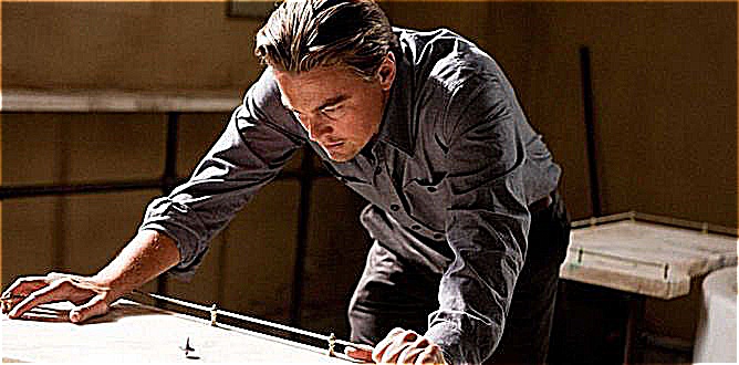
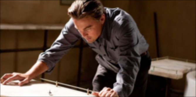
Inception: Original Sharp, Blurred, and Re-Sharpened
Here we evaluate the unsharp masking technique by taking a sharp image, blurring it, and then attempting to sharpen it again. We compare the original sharp image, the blurred version, and the sharpened result.

Part 2.2: Hybrid Images
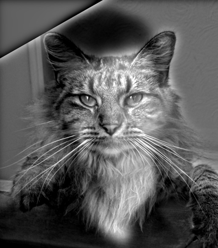
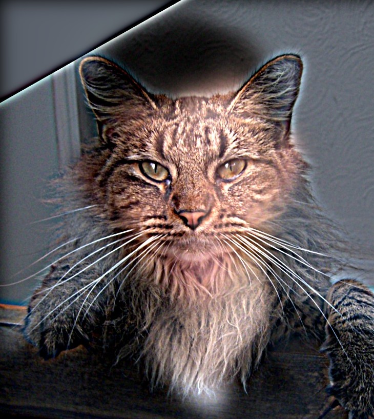
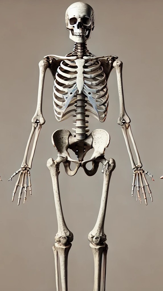
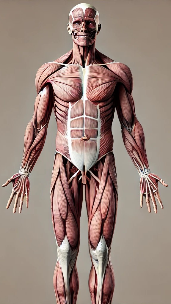
In this section, we create hybrid images using the method described in the SIGGRAPH 2006 paper by Oliva, Torralba, and Schyns. Hybrid images combine the high-frequency components of one image with the low-frequency components of another. The resulting images show different visual content depending on the viewing distance.
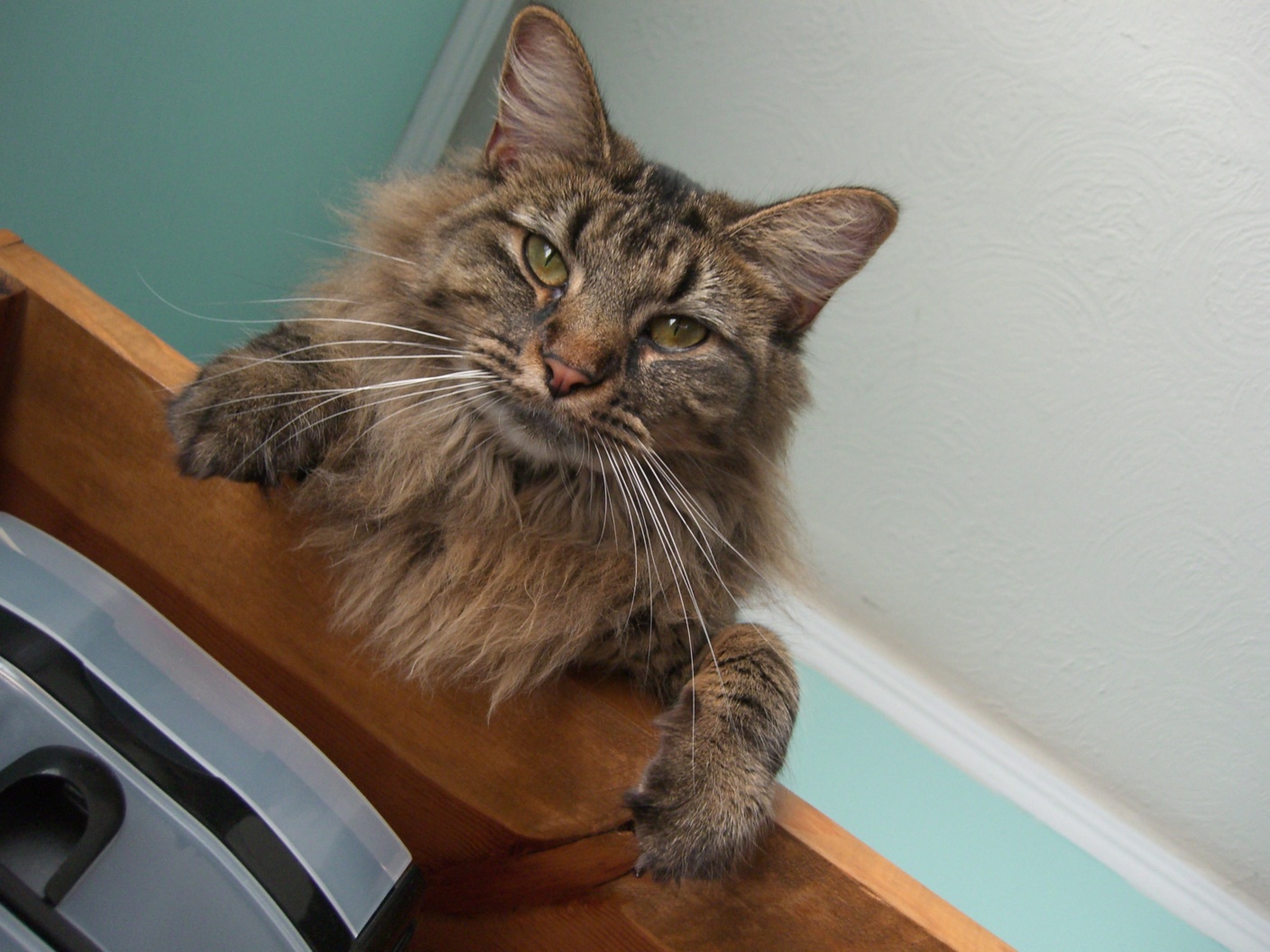
Derek and Nutmeg: Hybrid Image Example
We begin by showing both the color and grayscale versions of Derek and Nutmeg as a reference for creating a hybrid image.

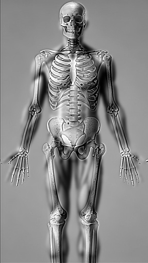
Skeleton and Muscle: Hybrid Image Example
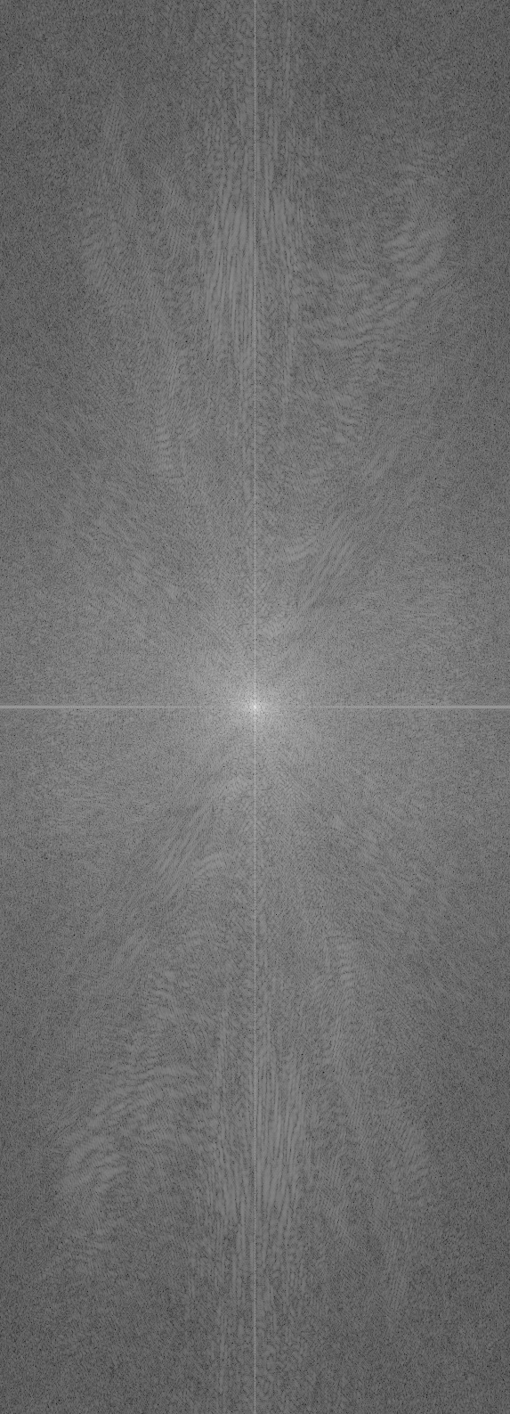
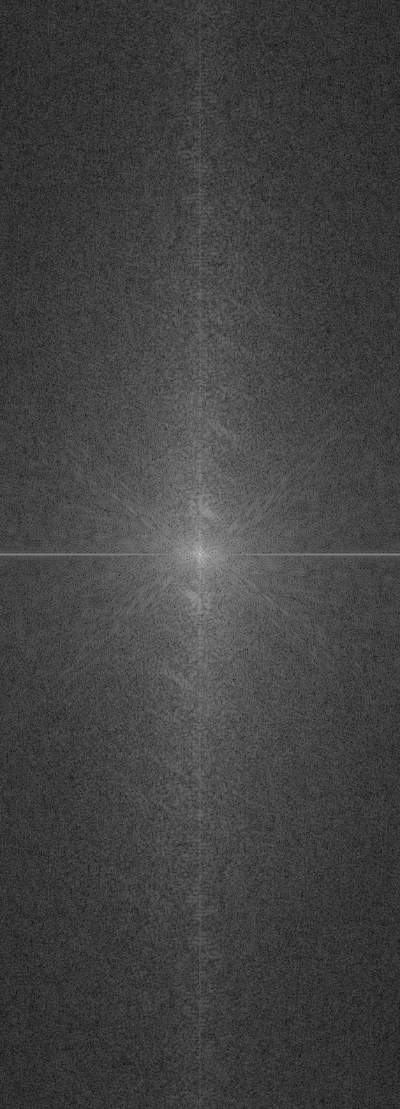
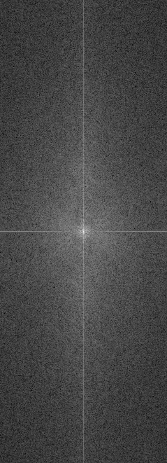
Next, we demonstrate the hybrid image creation with a pair of skeleton and muscle images. Below are the color versions followed by the grayscale versions with their corresponding frequency domain representations.
Grayscale and Frequency Analysis
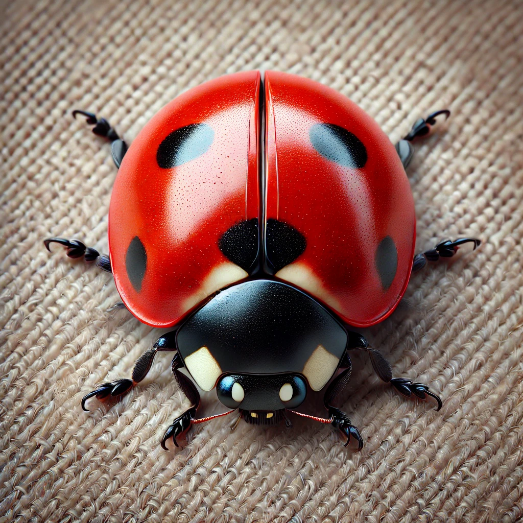
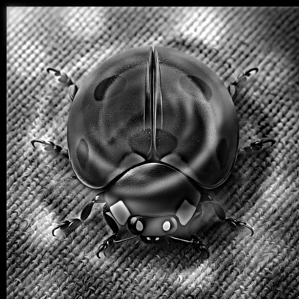
Flower and Ladybug: Hybrid Image Example
Lastly, we combine a flower and a ladybug image to create a hybrid image. Below are the original color images, followed by the grayscale versions and the final hybrid image.

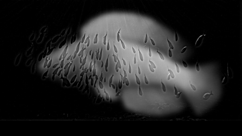
Fish and Ocean: Hybrid Image Example
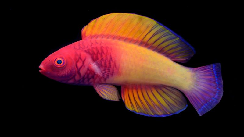
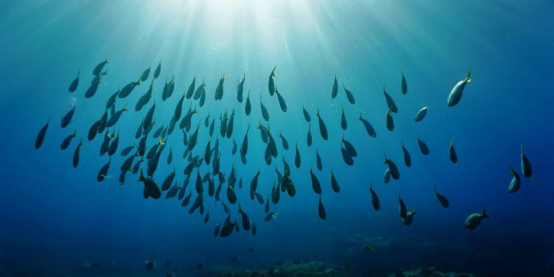
However, we can't always create hybrid images easily. There are several reasons as to why we can't easily make hybrid between two images. In this example of Fish and Ocean, we have lack of complexity between two images, as well as lack of visual contrast. This means when creating the low-pass and high-pass filter, we run into trouble as they overlap easily. So it becomes hard to distinguish the images
Part 2.3: Gaussian and Laplacian Stacks
In this section, we implemented Gaussian and Laplacian stacks to prepare for multi-resolution blending. These stacks maintain the same resolution at each level, unlike pyramids where images are downsampled. Below are the results of applying the Gaussian and Laplacian stacks to the Oraple (apple and orange blend).
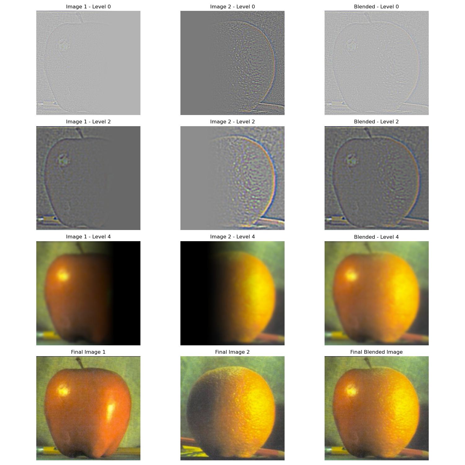
Oraple Blended using Laplacian Stack
Below is the blended result of the Oraple using Gaussian and Laplacian stacks to create a seamless transition between the apple and orange images.
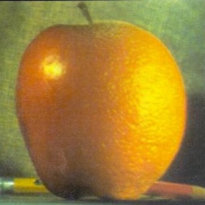
Part 2.4: Multiresolution Blending (The Oraple!)
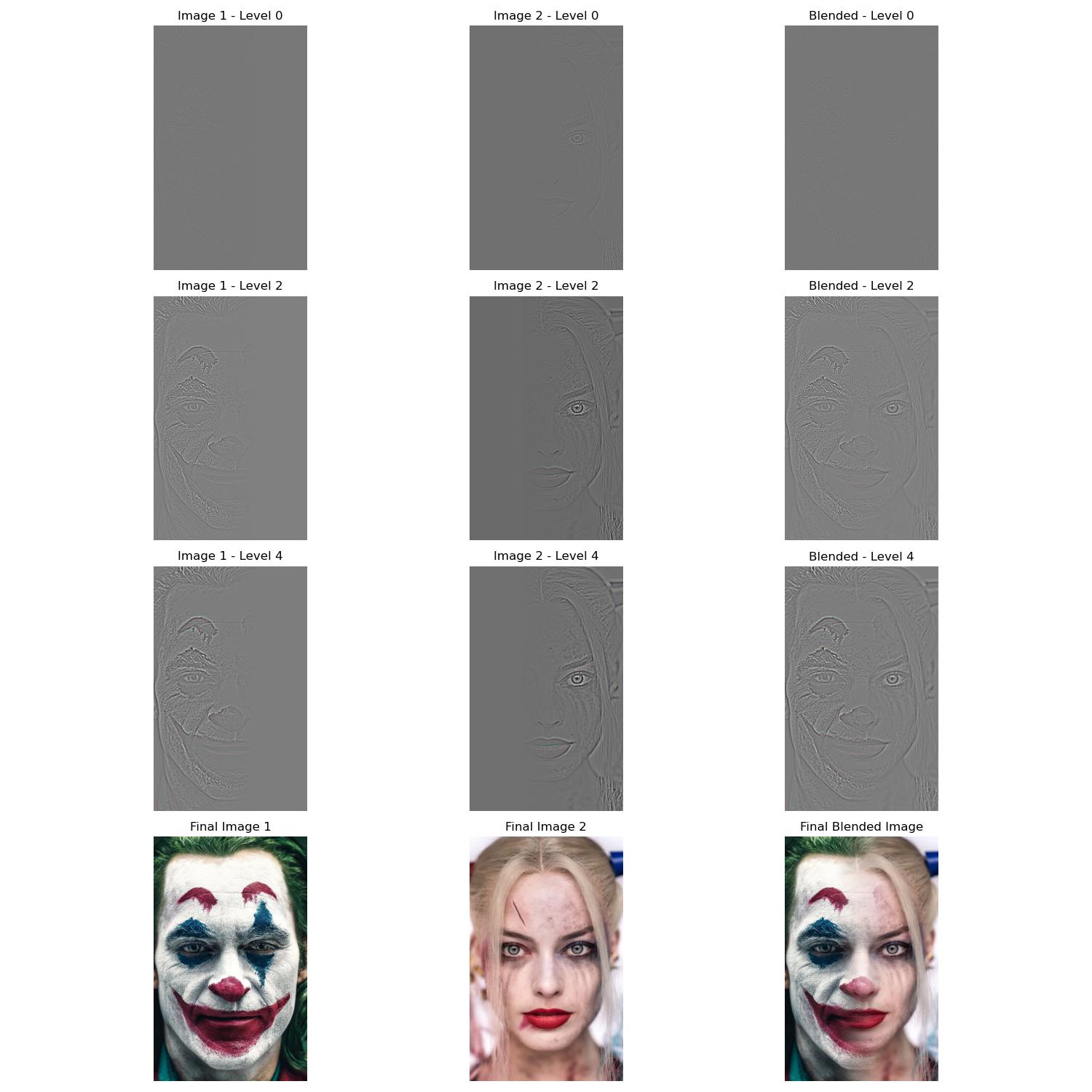
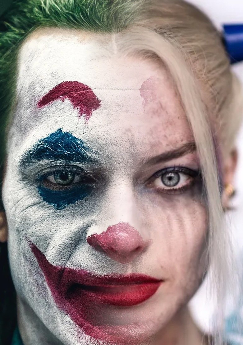
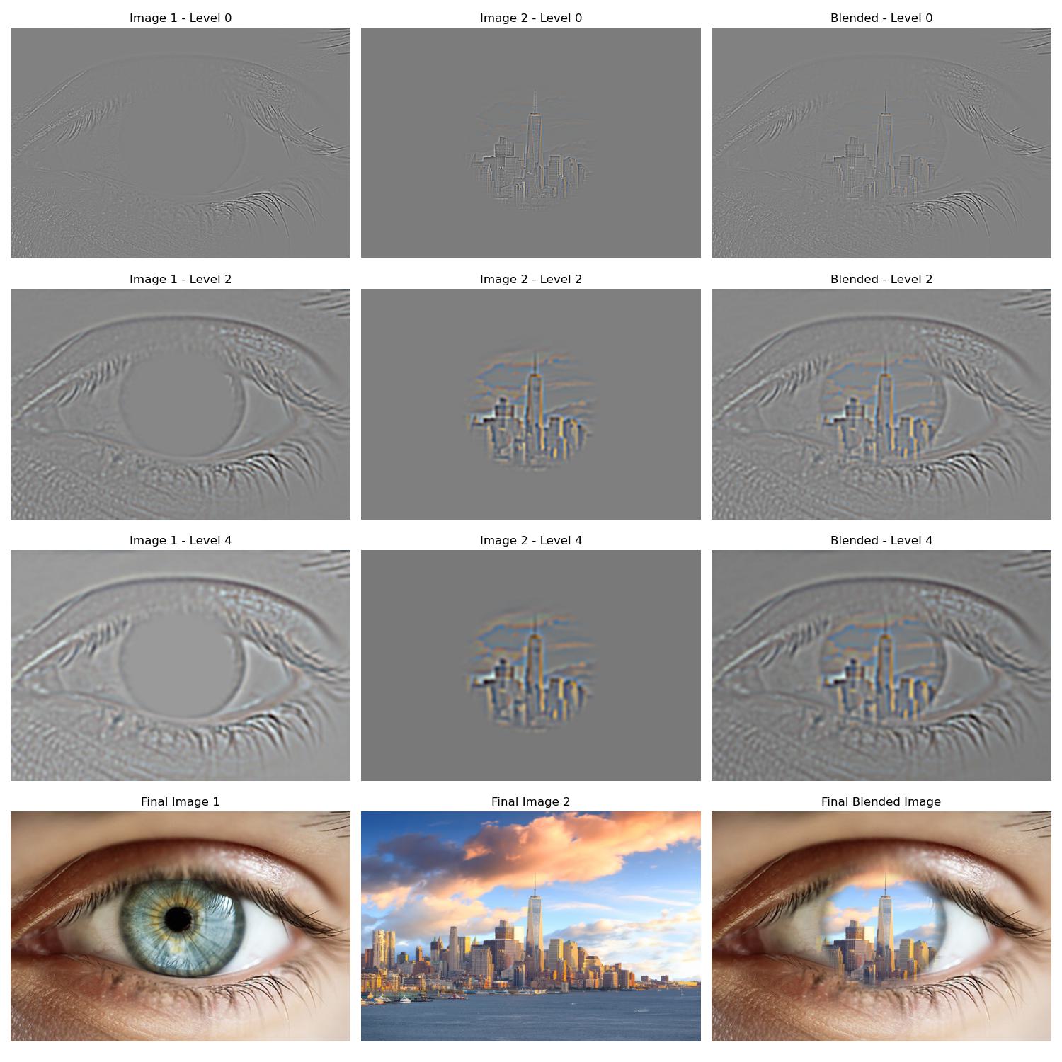
In this section, we applied multiresolution blending techniques to seamlessly merge two images using Gaussian and Laplacian stacks, inspired by the 1983 paper by Burt and Adelson. We started with the classic example of blending an apple and an orange (the Oraple), and then experimented with blending other creative image pairs.
Creative Image Blending Examples
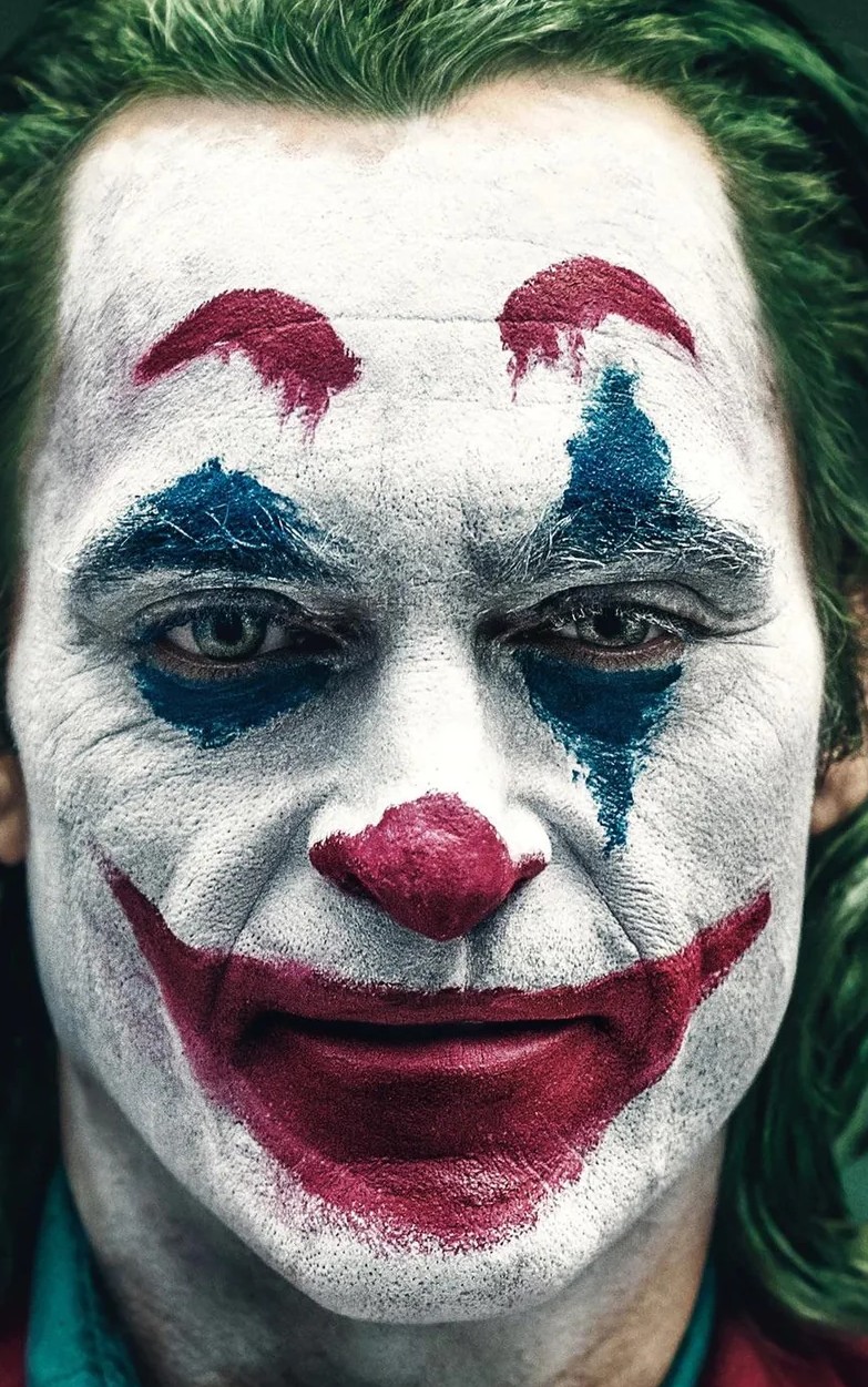
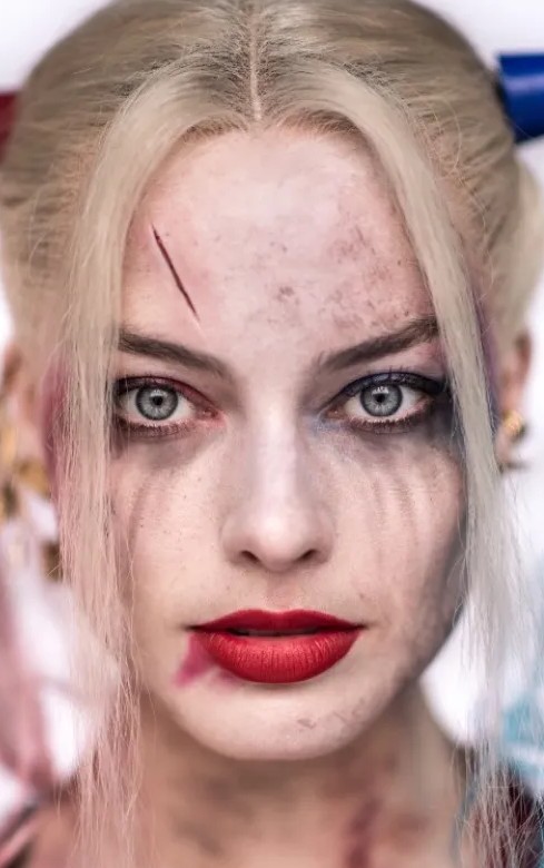
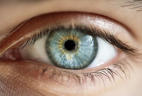
We experimented with blending two other image pairs using irregular masks for more creative results. Below are some examples:
