Project 5: Fun With Diffusion Models!
This project explores the application of diffusion models to generate and denoise images. The project is divided into two main parts:
- Part A: Playing with pre-trained diffusion models for tasks such as inpainting and optical illusions.
- Part B: Training your own diffusion model on the MNIST dataset.
Part A: Exploring Diffusion Models
In this part, you will explore the capabilities of pre-trained diffusion models, implement sampling loops, and use the models for tasks such as inpainting and generating optical illusions.
1.1 Implementing the Forward Process
The forward diffusion process adds Gaussian noise to an image over a series of timesteps \( t \), gradually corrupting the image. Mathematically, this is defined as:
\( x_t = \sqrt{\bar{\alpha}_t} \, x_0 + \sqrt{1 - \bar{\alpha}_t} \, \epsilon \),
where:
- \( x_t \): Noisy image at timestep \( t \).
- \( x_0 \): Clean original image.
- \( \bar{\alpha}_t \): Cumulative noise coefficient at \( t \).
- \( \epsilon \sim \mathcal{N}(0, I) \): Random Gaussian noise.
Below, we show a clean test image and its noisy counterparts at timesteps \( t = 250, 500, 750 \):

As the timestep \( t \) increases, the image becomes progressively noisier, with \( t = 750 \) being almost indistinguishable from pure noise.
1.2 Classical Denoising
In this part, we attempt to denoise the noisy images generated in the forward process (\( t = 250, 500, 750 \)) using classical Gaussian blur filtering. Gaussian blur reduces high-frequency noise by averaging nearby pixels, which is mathematically represented as:
\( G(x, y) = \sum_{i=-k}^{k} \sum_{j=-k}^{k} I(x+i, y+j) \cdot w(i, j) \),
where \( w(i, j) \) is the Gaussian kernel, and \( k \) is determined by the kernel size. Below, we show a comparison between the noisy images and their Gaussian-denoised counterparts for three timesteps:
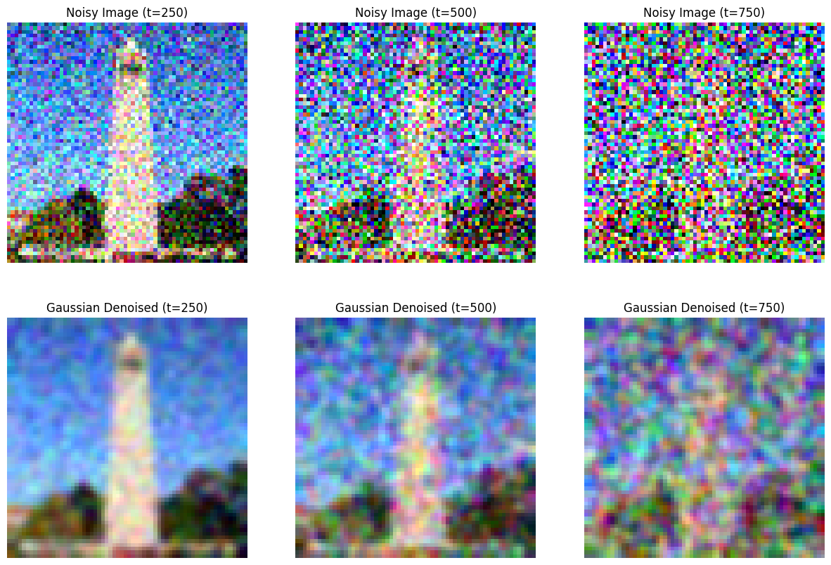
Observations: While Gaussian blur effectively smooths high-frequency noise, it also removes fine details from the image. At lower noise levels (\( t = 250 \)), some recognizable features remain visible. However, at higher noise levels (\( t = 750 \)), the denoised images still resemble smoothed noise, highlighting the limitations of classical methods in denoising structured diffusion noise.
1.3 Implementing One Step Denoising
In this section, we use a pretrained diffusion model (DeepFloyd's stage_1.unet) to estimate and remove noise from noisy images. The process involves three steps:
- Estimate the noise \( \hat{\epsilon} \) in the noisy image \( x_t \).
- Remove the noise using the estimated noise and timestep-specific parameters.
- Recover an estimate of the original image \( x_0 \).
The forward diffusion process adds Gaussian noise to an image, as defined by:
\( x_t = \sqrt{\bar{\alpha}_t} \, x_0 + \sqrt{1 - \bar{\alpha}_t} \, \epsilon \),
where:
- \( x_t \): Noisy image at timestep \( t \).
- \( x_0 \): Clean original image.
- \( \bar{\alpha}_t \): Cumulative noise coefficient.
- \( \epsilon \): Random Gaussian noise.
The pretrained UNet estimates the noise \( \hat{\epsilon} \) in \( x_t \). Using this noise estimate, the original image \( x_0 \) is recovered by reversing the forward process:
\( x_0 \approx \frac{x_t - \sqrt{1 - \bar{\alpha}_t} \, \hat{\epsilon}}{\sqrt{\bar{\alpha}_t}} \).
Below, we visualize the original image, the noisy image at timesteps \( t = 250, 500, 750 \), and the recovered estimate \( x_0 \):


Observations:
- For \( t = 250 \), the recovered image closely resembles the original image, as the noise level is relatively low.
- For \( t = 500 \), the recovered image retains some structure but starts losing finer details.
- For \( t = 750 \), the recovered image is less accurate, as the noise overwhelms the signal.
1.4 Implementing Iterative Denoising
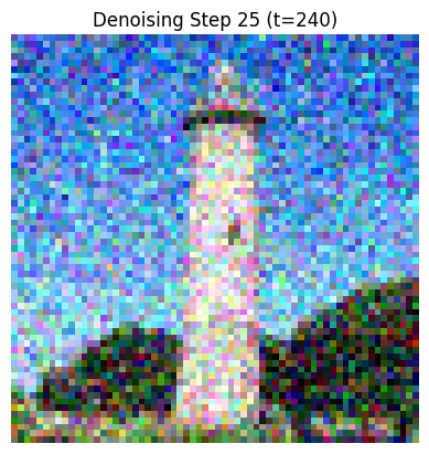
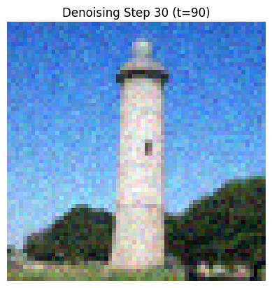
In this section, we implement and evaluate an iterative denoising process using the pretrained DeepFloyd diffusion model. Iterative denoising progressively reduces noise by moving from a noisy image \( x_t \) at a timestep \( t \) to a less noisy image \( x_{t'} \), until a clean image \( x_0 \) is obtained. The timesteps \( t \) are selected from a list of strided timesteps, starting at \( t = 990 \) and ending at \( t = 0 \) in steps of 30.
The denoising process for a single step is governed by the formula:
\( x_{t'} = \frac{\sqrt{\bar{\alpha}_{t'}} \, \beta_t}{1 - \bar{\alpha}_t} \, x_0 + \frac{\sqrt{\alpha_t} \, (1 - \bar{\alpha}_{t'})}{1 - \bar{\alpha}_t} \, x_t + v_\sigma \),
where:
- \( x_{t'} \): The less noisy image at timestep \( t' \).
- \( x_0 \): Current estimate of the clean image.
- \( v_\sigma \): Variance noise, added using the provided
add_variancefunction.
Below, we visualize the iterative denoising process, starting from \( t = 300 \) and gradually reducing noise until \( t = 0 \).
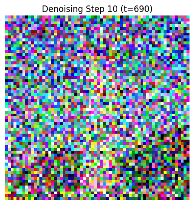
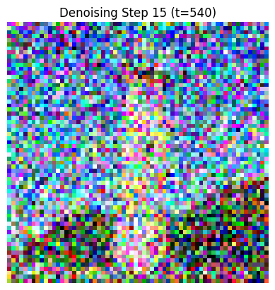
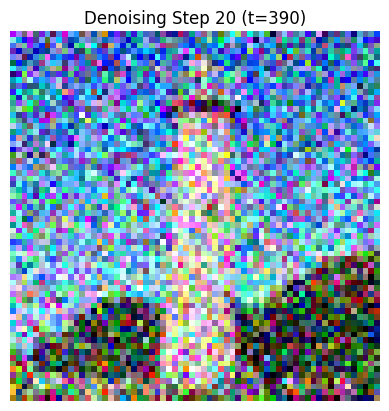

Key Observations:
- Iterative Denoising: The final clean image is significantly closer to the original, as noise is removed progressively at each step.
- One-Step Denoising: This method is less effective, as it attempts to denoise all at once, leading to incomplete noise removal.
- Gaussian Blurring: This classical approach smooths high-frequency noise but cannot handle structured noise, resulting in blurry images.
1.5 Diffusion Model Sampling
In this section, we use the pretrained diffusion model to generate images from scratch. Starting with pure Gaussian noise, the model iteratively denoises the noise step-by-step until a coherent image is obtained. This process leverages the pretrained UNet's ability to map noise to the manifold of natural images, conditioned on the prompt "a high quality photo."
The process begins with pure noise \( x_T \) at the noisiest timestep \( t = 990 \). Iterative denoising then progressively reduces noise using the following formula:
\( x_{t'} = \frac{\sqrt{\bar{\alpha}_{t'}} \, \beta_t}{1 - \bar{\alpha}_t} \, x_0 + \frac{\sqrt{\alpha_t} \, (1 - \bar{\alpha}_{t'})}{1 - \bar{\alpha}_t} \, x_t + v_\sigma \),
where:
- \( x_{t'} \): Image at the next timestep \( t' \), closer to a clean image.
- \( x_0 \): Estimated clean image at the current step.
- \( v_\sigma \): Variance noise added during the denoising process.
Below, we display 5 sampled images generated by the model using this method:

1.6 Classifier-Free Guidance (CFG)
In this section, we use Classifier-Free Guidance (CFG) to improve the quality of generated images. CFG combines both conditional and unconditional noise estimates to guide the generation process. The noise estimate is defined as:
\( \epsilon = \epsilon_u + \gamma (\epsilon_c - \epsilon_u) \),
where:
- \( \epsilon_u \): Unconditional noise estimate (null prompt).
- \( \epsilon_c \): Conditional noise estimate (prompt: "a high quality photo").
- \( \gamma \): CFG scale, controlling the strength of guidance (\( \gamma = 7 \) in this example).
During the iterative denoising process:
- The UNet computes \( \epsilon_c \) by conditioning on the prompt embedding.
- It computes \( \epsilon_u \) by conditioning on a null embedding.
- Using the formula above, a guided noise estimate \( \epsilon \) is calculated.
- The image is progressively refined using the CFG-modified estimate until it converges to a visually coherent result.
Below are 5 images generated using CFG with a scale of \( \gamma = 7 \):

Key Observations:
- By amplifying the conditional signal (\( \gamma > 1 \)), CFG produces images that are more aligned with the prompt and exhibit significantly improved quality compared to earlier methods.
- The use of unconditional noise estimates (\( \epsilon_u \)) ensures a balance between diversity and fidelity in the generated outputs.
- The computational cost is higher as the UNet must compute both \( \epsilon_c \) and \( \epsilon_u \) for every timestep.
1.7 Image-to-Image Translation
In this section, we explore the process of Image-to-Image Translation, where we take a real image, add varying levels of noise, and iteratively denoise it using the diffusion model. This technique, inspired by the SDEdit algorithm, allows the model to make edits to an image by forcing it back onto the manifold of natural images.
The forward process adds noise to the image:
\( x_t = \sqrt{\bar{\alpha}_t} \, x_0 + \sqrt{1 - \bar{\alpha}_t} \, \epsilon \),
where:
- \( x_t \): Noisy image at timestep \( t \).
- \( x_0 \): Clean original image.
- \( \bar{\alpha}_t \): Cumulative noise coefficient at \( t \).
- \( \epsilon \sim \mathcal{N}(0, I) \): Random Gaussian noise.
The noisy image \( x_t \) is then denoised iteratively using Classifier-Free Guidance (CFG):
\( \epsilon = \epsilon_u + \gamma (\epsilon_c - \epsilon_u) \),
where:
- \( \epsilon_c \): Conditional noise estimate (prompt: "a high quality photo").
- \( \epsilon_u \): Unconditional noise estimate (prompt: "").
- \( \gamma = 7 \): CFG scale, controlling the strength of guidance.
Below, we show the progression of edits for:
- The original test image at noise levels \( t = [1, 3, 5, 7, 10, 20] \).
- Two custom images ("dogs" and "eskimo") using the same procedure.


Observations:
- At low noise levels (e.g., \( t = 1, 3 \)), the edited image closely resembles the original image, with minimal changes.
- At higher noise levels (e.g., \( t = 10, 20 \)), the model exhibits more creativity, hallucinating additional details or changes.
- The approach demonstrates the flexibility of diffusion models for editing images based on noise levels and denoising strength.
1.7.1 Editing Hand-Drawn and Web Images
In this section, we explore how the SDEdit algorithm can project non-realistic images, such as paintings, sketches, and web images, onto the natural image manifold. The method involves adding noise at specific levels (\( t = [1, 3, 5, 7, 10, 20] \)) and iteratively denoising the image using Classifier-Free Guidance (CFG).
The forward process adds noise using:
\( x_t = \sqrt{\bar{\alpha}_t} \, x_0 + \sqrt{1 - \bar{\alpha}_t} \, \epsilon \),
and the CFG-adjusted noise estimate for denoising is given by:
\( \epsilon = \epsilon_u + \gamma (\epsilon_c - \epsilon_u) \),
where:
- \( \epsilon_c \): Noise estimate conditioned on the text prompt.
- \( \epsilon_u \): Unconditional noise estimate (no prompt).
- \( \gamma = 7 \): CFG scale, which controls the strength of guidance.
Web Image: Minions
The selected web image of "Minions" was processed using the SDEdit algorithm. Noise was added at timesteps \( t = [1, 3, 5, 7, 10, 20] \), and the model iteratively denoised the noisy image back to the natural image manifold. Below are the results:


Hand-Drawn Images: A Fish and Phineas
Two hand-drawn images, "A Fish" and "Phineas," were created and processed using the same method. Noise levels \( t = [1, 3, 5, 7, 10, 20] \) were applied, and iterative denoising with CFG was used to refine the images. The results showcase how the diffusion model creatively transforms these inputs into realistic outputs while retaining artistic characteristics.


Observations:
- The "Minions" web image was effectively refined, retaining its overall structure while aligning with the "a high quality photo" prompt.
- The hand-drawn images, "A Fish" and "Phineas," were creatively projected onto the natural image manifold, showcasing the model's ability to refine and enhance non-realistic inputs.
1.7.2 Inpainting
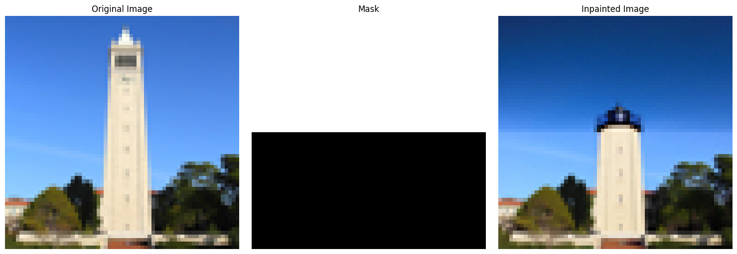
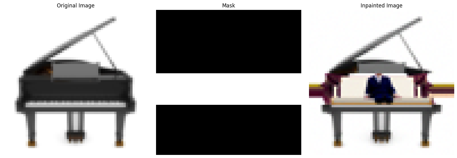
In this section, we explore the capability of diffusion models for inpainting. Inpainting involves editing specific parts of an image while preserving other regions. Using a binary mask \( m \), where \( m = 1 \) represents the areas to edit and \( m = 0 \) represents areas to preserve, the model refines the noisy regions back to the natural image manifold.
The inpainting process follows the formula:
\( x_t \leftarrow m x_t + (1 - m) \text{forward}(x_{\text{orig}}, t) \)
This ensures that pixels outside the mask retain their original values with appropriate noise, while pixels inside the mask are denoised iteratively. The model progressively refines the image using the iterative denoising process.
Test Image: Inpainting with a Rectangular Mask
Below, we demonstrate inpainting on the test image with a rectangular mask that targets the top half of the image. The mask ensures that only the top portion is edited while the rest remains unchanged:
Custom Image 1: Piano (Rectangular Mask)
For the piano image, we applied a rectangular mask that spans the middle section of the image. This mask allows the model to focus its edits on that region, leaving the rest of the image untouched:
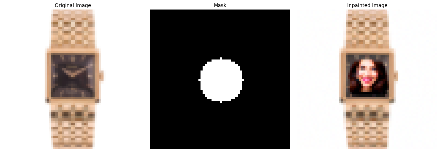
Custom Image 2: Rolex (Circular Mask)
For the Rolex image, we used a circular mask centered in the middle of the image. The circular mask allows the model to refine the specific region within the circle, while preserving the outer area as is:
1.7.3 Text-Conditioned Image-to-Image Translation
In this section, we use text-conditioned embeddings to guide the image projection process onto the natural image manifold. By changing the prompt from "a high quality photo" to a specific text description, we add control using language. For instance, we used the prompt "a rocket ship" to guide the denoising process.
The iterative denoising process is guided by the classifier-free guidance (CFG) scale \( \gamma \), which was set to \( \gamma = 7 \). This process was applied to the test image and two custom images, namely an orchestra and an F1 race.
Edits of the Test Image
The following results show the test image progressively edited at noise levels [1, 3, 5, 7, 10, 20]:

Edits of Custom Image 1: Orchestra
Below are the results of applying the same procedure on the orchestra image:

Edits of Custom Image 2: F1 Race
Finally, we applied the text-conditioned translation to an image of an F1 race:

Part 1.8: Visual Anagrams
In this section, we implemented visual anagrams using a diffusion model. A visual anagram is an image that appears as one subject when upright and as another subject when flipped upside down. This effect was achieved by conditioning the denoising process on two different text prompts and averaging the noise estimates from both orientations during iterative denoising.
Mathematically, the algorithm for noise estimation is:
\( \epsilon_1 = \text{UNet}(x_t, t, p_1) \), \( \epsilon_2 = \text{flip}(\text{UNet}(\text{flip}(x_t), t, p_2)) \),
\( \epsilon = \frac{\epsilon_1 + \epsilon_2}{2} \),
where \( p_1 \) and \( p_2 \) are the text prompt embeddings, and \( \text{flip}(\cdot) \) represents vertical flipping. The final denoising process uses this averaged noise estimate to iteratively refine the image.
Deliverables
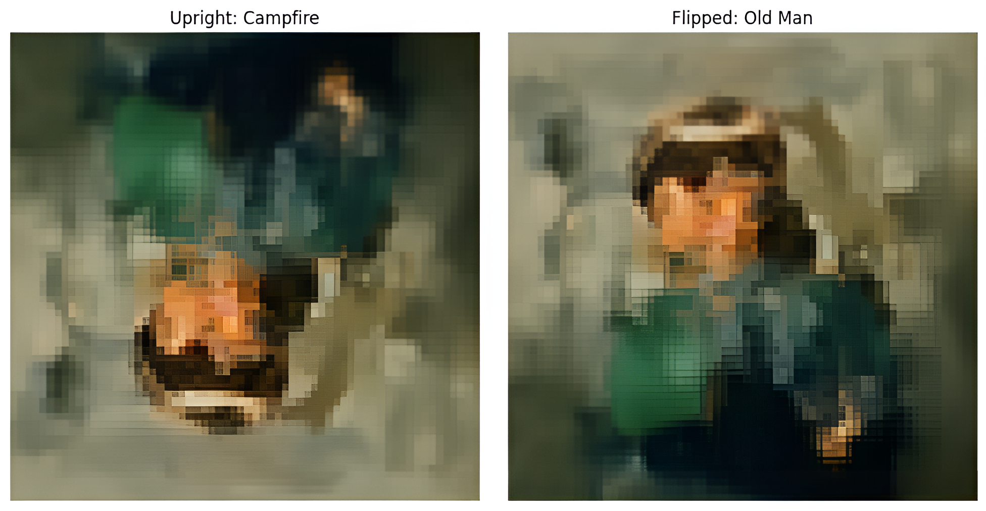
1. Visual Anagram: "Campfire" and "Old Man"
This visual anagram appears as "an oil painting of people around a campfire" when upright and "an oil painting of an old man" when flipped upside down:
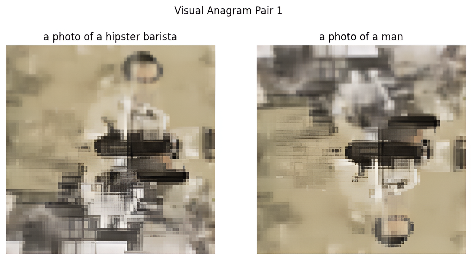
2. Visual Anagram: "Hipster Barista" and "Man"
This visual anagram appears as "a photo of a hipster barista" when upright and "a photo of a man" when flipped upside down:
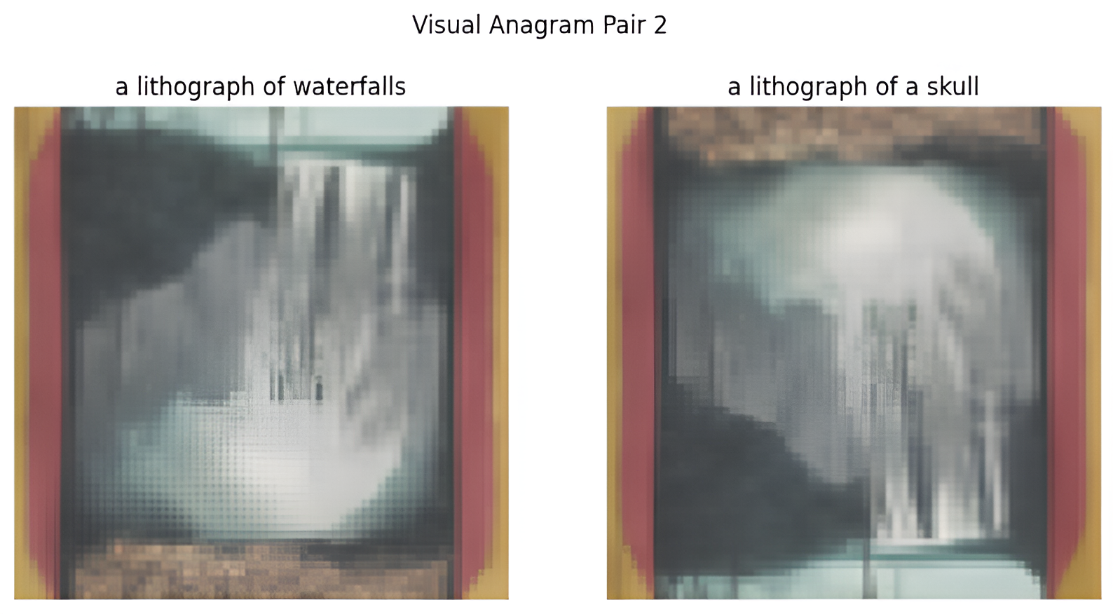
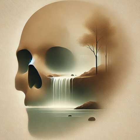
3. Visual Anagram: "Waterfalls" and "Skull"
This visual anagram appears as "a lithograph of waterfalls" when upright and "a lithograph of a skull" when flipped upside down:
Explanation
To create these illusions, the following steps were performed:
- Initialize a random noise image \( x_t \) at timestep \( t=1000 \).
- Iteratively denoise the image using the text prompt for the upright orientation while simultaneously flipping the image vertically and denoising with the flipped prompt.
- Averaged the noise estimates from both orientations and used the result to guide the next denoising step.
- Displayed the final upright and flipped images to demonstrate the illusion.
Part A: Exploring Diffusion Models
1.9 Hybrid Images
In this section, we created hybrid images that appear as one image from far away (low frequency) and a different image up close (high frequency). The results leverage Gaussian blur to isolate low-frequency components and combine them with the high-frequency details of another prompt.
The hybrid image creation process involves iterative denoising guided by two separate text prompts for the far and close views, blending their frequency components to create a visually striking effect. The formula used for combining the images is:
\( \text{Hybrid Image} = \text{Low Frequency Image} + (\text{High Frequency Image} - \text{Blurred High Frequency Image}) \)
Below are the results for three hybrid images:
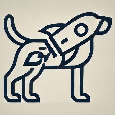

How it Works
To create these images:
- We started with pure noise and denoised it iteratively using a combination of low-frequency and high-frequency components guided by separate text prompts.
- Gaussian blur was applied to isolate the low-frequency components for the far view.
- High-frequency components were preserved by subtracting the blurred high-frequency image from the original high-frequency image.
- The two frequency components were combined to create the final hybrid image.
Observations
Each hybrid image effectively combines the visual properties of two different prompts. From far away, the low-frequency image dominates, creating the appearance of the first prompt. As you get closer, the high-frequency details become visible, revealing the second prompt.
Part B: Training Your Own Diffusion Model
In this part, we train a UNet-based diffusion model on the MNIST dataset. The process involves generating noisy images, training the model to denoise them, and evaluating the model’s performance.
Part 1: Visualization of the Noising Process
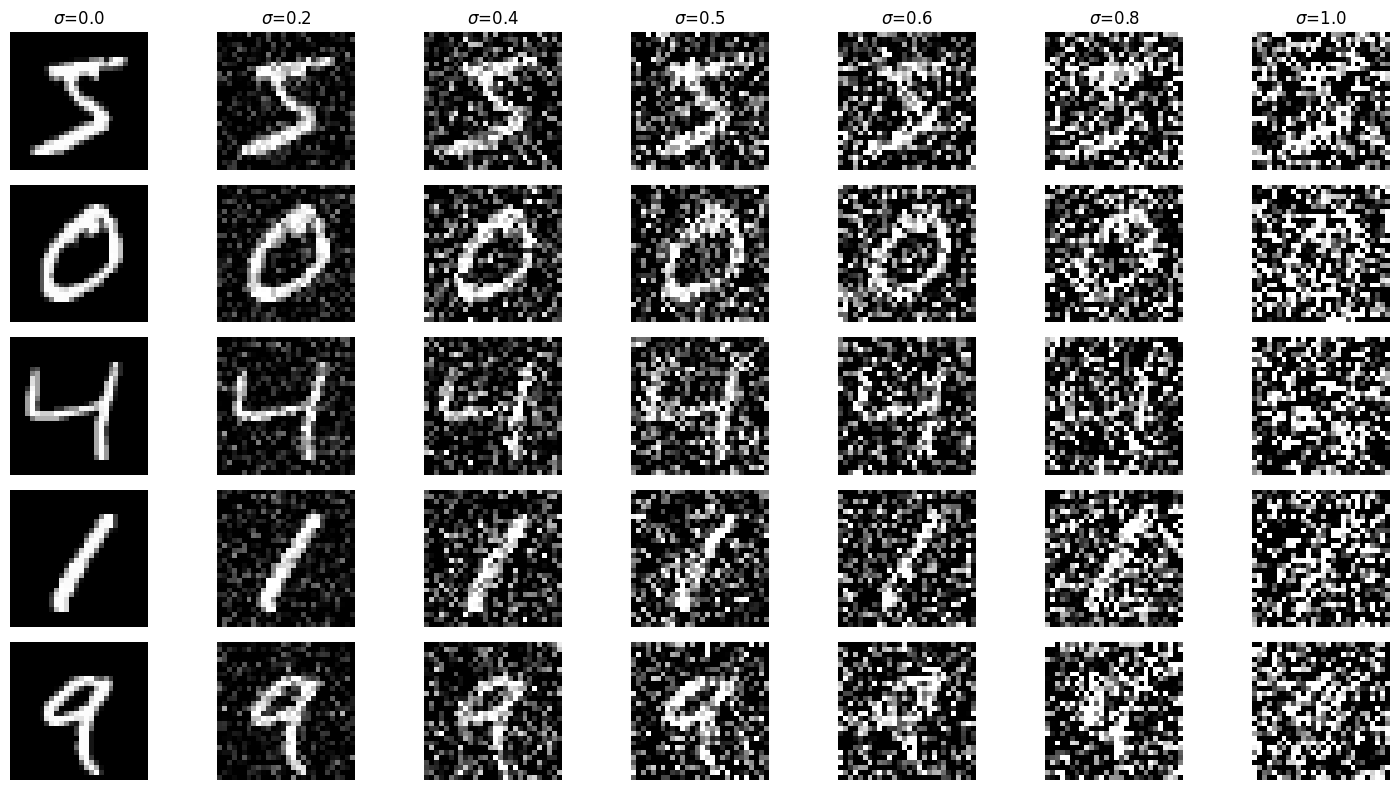
To train the UNet denoiser, we generate noisy images \( z \) by adding Gaussian noise to clean MNIST images \( x \), as follows:
z = x + σ * ε, where ε ∼ N(0, I).
Below is a visualization of the noising process, showing how images are progressively corrupted as the noise level \( \sigma \) increases:
Part 2: Training Loss Curve
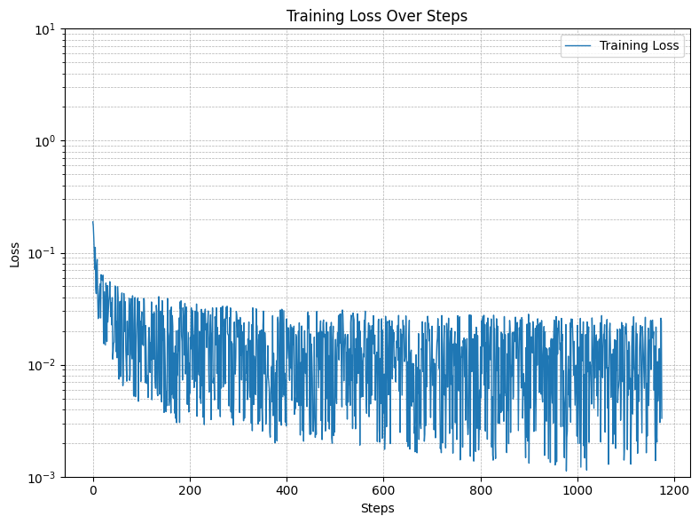
The UNet denoiser was trained to minimize the L2 loss:
\( L = \mathbb{E}_{z,x} [\| D_\theta(z) - x \|^2] \)
Training was conducted over 5 epochs, with random noise levels applied to the images during each batch. The following plot shows the training loss over steps:
Part 3: Sample Results on the Test Set
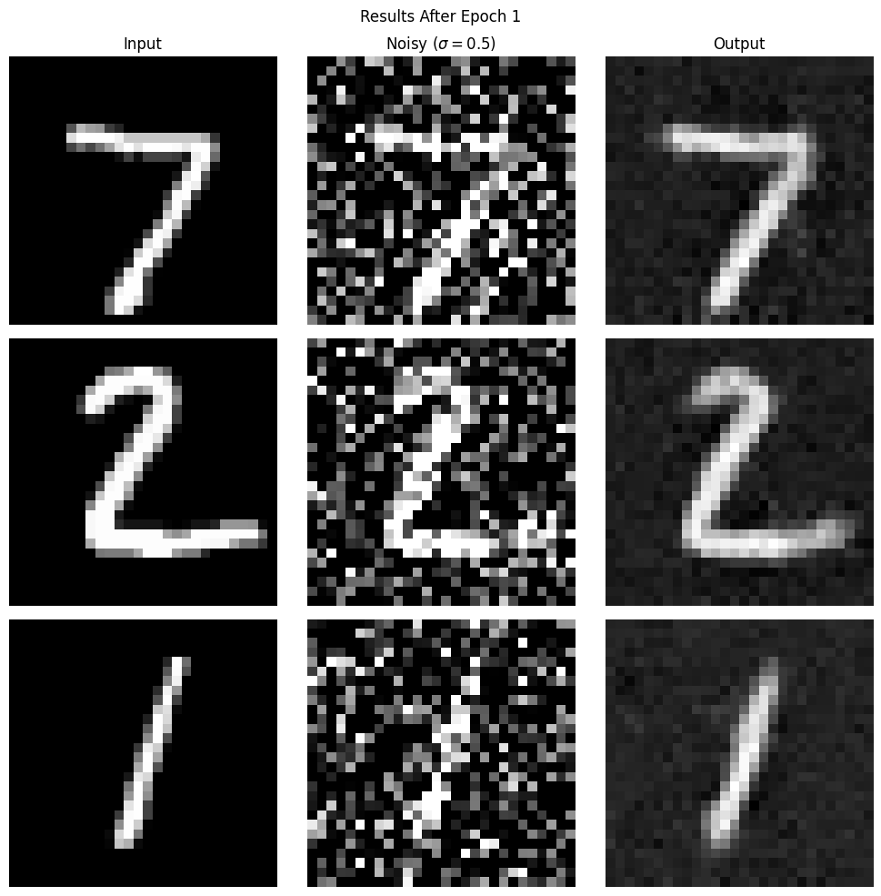
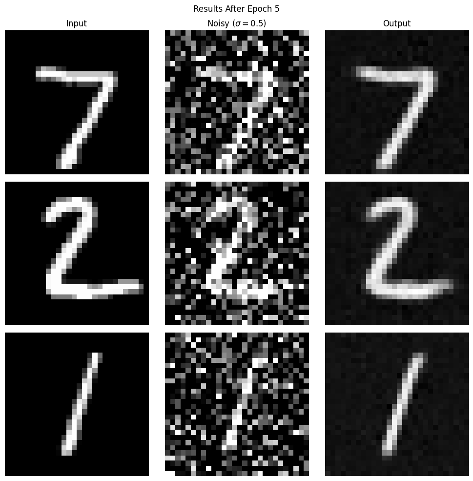
After training, the denoiser was tested on unseen MNIST digits. Below are the results of the denoiser:
- After the 1st Epoch: Early-stage denoising results.
- After the 5th Epoch: Final denoising performance.
Part 4: Out-of-Distribution Testing
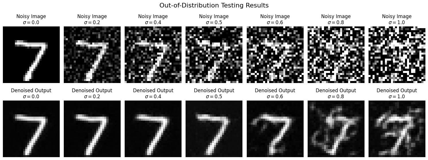
To evaluate the model's generalization, the denoiser was tested on noise levels it was not trained for, ranging from \( \sigma = [0.0, 0.2, 0.4, 0.5, 0.6, 0.8, 1.0] \). The results below show how the model performs as the noise level increases:
Part 2: Training a Time-Conditioned UNet
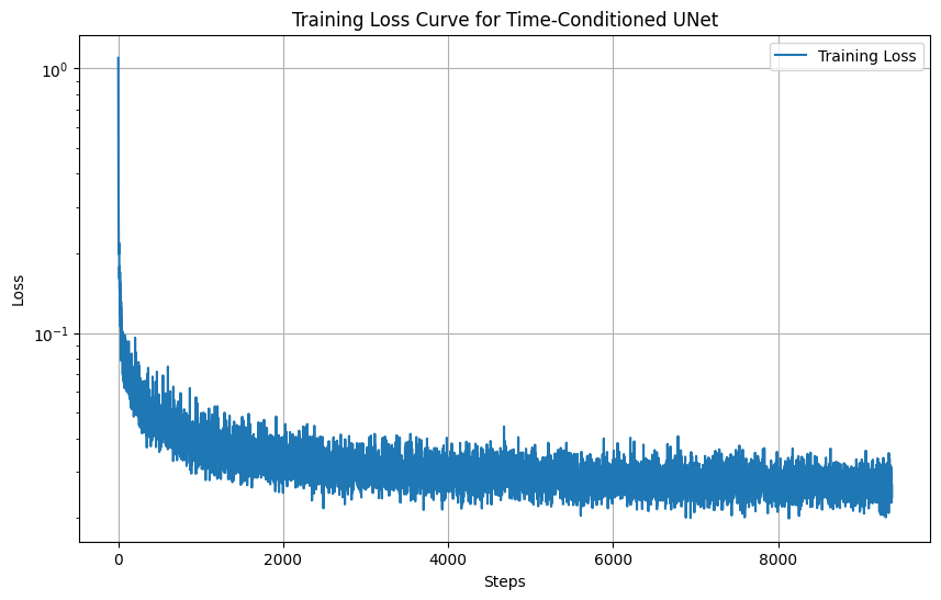
Training Loss Curve
To train the time-conditioned UNet \( \epsilon_\theta(x_t, t) \), we minimize the L2 loss:
\( L = \mathbb{E}_{x_0, t, \epsilon} \| \epsilon_\theta(x_t, t) - \epsilon \|^2 \)
Here:
- \( x_0 \): Clean image from the training set.
- \( t \): Random timestep sampled from \( \{1, \dots, T\} \).
- \( \epsilon \sim \mathcal{N}(0, I) \): Gaussian noise added to the image.
Sampling Results
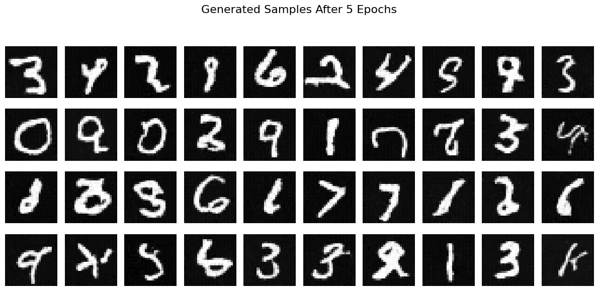
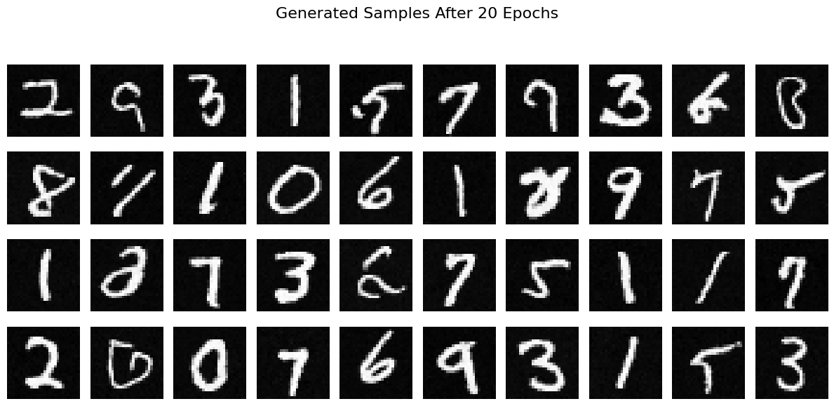
Using the trained UNet, we generate images by iteratively denoising a pure noise image \( x_T \sim \mathcal{N}(0, I) \) through the reverse diffusion process. The equations for denoising are as follows:
\( x_t = \sqrt{\bar{\alpha}_t} x_0 + \sqrt{1 - \bar{\alpha}_t} \epsilon \)
At each timestep \( t \), the UNet predicts the noise \( \epsilon_\theta(x_t, t) \), which is used to compute the denoised image \( x_0 \):
\( x_0 = \frac{1}{\sqrt{\bar{\alpha}_t}} \left( x_t - \sqrt{1 - \bar{\alpha}_t} \epsilon_\theta(x_t, t) \right) \)
Then, the next timestep \( x_{t-1} \) is computed as:
\( x_{t-1} = \frac{\sqrt{\bar{\alpha}_{t-1}}}{\sqrt{1 - \bar{\alpha}_t}} x_0 + \frac{\sqrt{\alpha_t} (1 - \bar{\alpha}_{t-1})}{1 - \bar{\alpha}_t} x_t + \sqrt{\beta_t} z \)
Here:
- \( z \sim \mathcal{N}(0, I) \) is Gaussian noise for \( t > 1 \), or \( z = 0 \) if \( t = 1 \).
- \( \bar{\alpha}_t \): Cumulative product of \( \alpha_t = 1 - \beta_t \).
Below are the generated images after 5 and 20 epochs of training. These results demonstrate the improvement in the UNet's ability to generate clean samples as training progresses.
Part 6: Class-Conditioned UNet Training and Sampling
Training Overview
In this section, we extend the UNet to be class-conditioned, allowing it to generate MNIST digits conditioned on their class (digits 0-9). This involves introducing class-conditioning vectors alongside time-conditioning. The model is trained using a combination of the class and time signals, with dropout applied to class-conditioning 10% of the time to enable unconditional generation.
The class-conditioned UNet minimizes the noise prediction loss:
\( L = \mathbb{E}_{x_0, t, c, \epsilon} \| \epsilon - \epsilon_\theta(x_t, t, c) \|^2 \)
where \( x_t \) is generated as:
\( x_t = \sqrt{\bar{\alpha}_t} x_0 + \sqrt{1 - \bar{\alpha}_t} \epsilon \)
Training details:
- Batch size: 128
- Learning rate: 1e-3
- Epochs: 20
- Unconditioning probability (\( p_{\text{uncond}} \)): 0.1
- Guidance scale (\( \gamma \)): 5.0
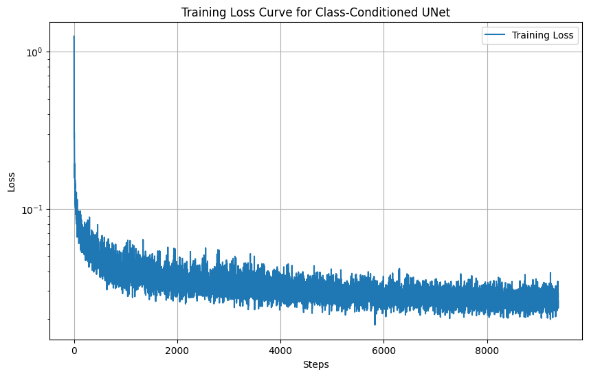
Below is the training loss curve, showing convergence over the course of training:
Sampling Overview
During sampling, we use classifier-free guidance to enhance the quality of class-conditioned results. The guided noise prediction is computed as:
\( \epsilon = \epsilon_u + \gamma (\epsilon_c - \epsilon_u) \)
where:
- \( \epsilon_u = \epsilon_\theta(x_t, t, 0) \) is the unconditional noise prediction.
- \( \epsilon_c = \epsilon_\theta(x_t, t, c) \) is the class-conditioned noise prediction.
- \( \gamma = 5.0 \) is the guidance scale.
The denoising process then follows the reverse diffusion formula:
\( x_0 = \frac{1}{\sqrt{\bar{\alpha}_t}} \left( x_t - \sqrt{1 - \bar{\alpha}_t} \epsilon \right) \)
\( x_{t-1} = \frac{\sqrt{\bar{\alpha}_{t-1}} \hat{x}_0}{1 - \bar{\alpha}_{t-1}} + \sqrt{\beta_t} z + \frac{\sqrt{\alpha_t} (1 - \bar{\alpha}_{t-1})}{1 - \bar{\alpha}_t} x_t \)
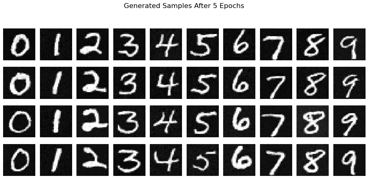
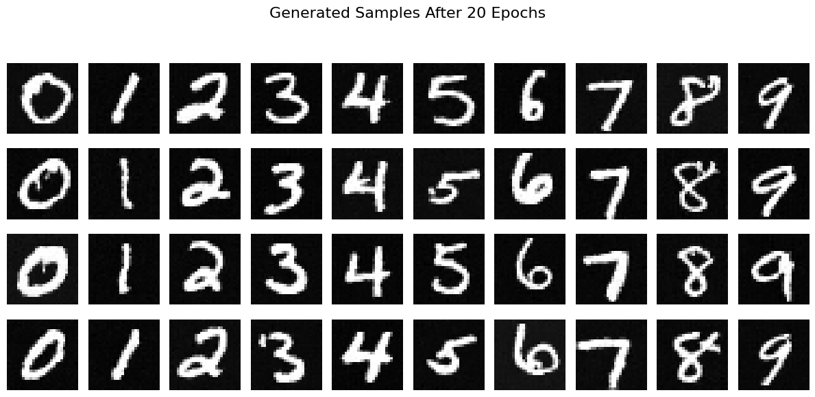
Sampling results for 4 instances of each digit (0-9) after 5 and 20 epochs of training are shown below:
Observations
The training loss curve indicates steady convergence over 20 epochs, suggesting that the UNet learns to predict noise effectively for both class-conditioned and unconditional generation. Sampling results show the improvement in generation quality and diversity after 20 epochs compared to 5 epochs.
Classifier-free guidance significantly enhances the quality of the generated images by leveraging both unconditional and class-conditioned predictions.