Neural Radiance Field Project
Part 1: Fitting a Neural Field to a 2D Image
Introduction
In this part of the Neural Radiance Field project, we create a neural field that maps 2D image coordinates to RGB values using a Multi-Layer Perceptron (MLP) and Sinusoidal Positional Encoding (PE). The model is trained to reconstruct an image by optimizing the network's parameters.
Model Architecture
The model used in this project is a Multi-Layer Perceptron (MLP) with the following configuration:
- Input Features: 2D coordinates with positional encoding (\(x, y\))
- Hidden Layers: 4 layers with 256 hidden units each
- Activation Function: ReLU for hidden layers
- Output Layer: Sigmoid function to constrain output RGB values to \([0, 1]\)
- Positional Encoding \(L\): 10
- Learning Rate: 0.01
The following diagram illustrates the architecture of the neural network:

Figure 1: MLP Architecture with Positional Encoding
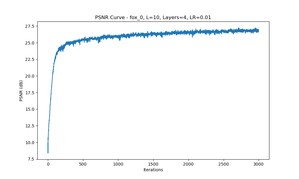
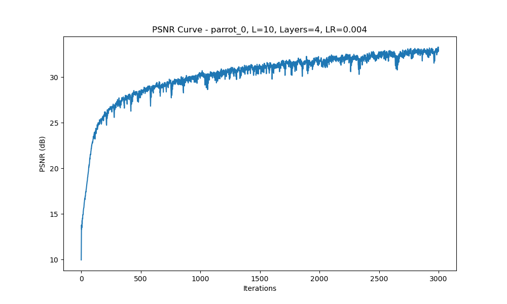
During training, we track the Peak Signal-to-Noise Ratio (PSNR) to measure the quality of the reconstruction. The plot below shows the PSNR across training iterations:

Figure 2: PSNR Curve Over Iterations
Training Process
The model is trained using Mean Squared Error (MSE) loss with the Adam optimizer. The training process involves randomly sampling pixels (batch size of 10,000) and optimizing the network to predict their RGB values.
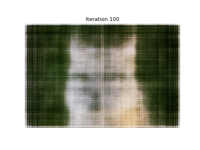
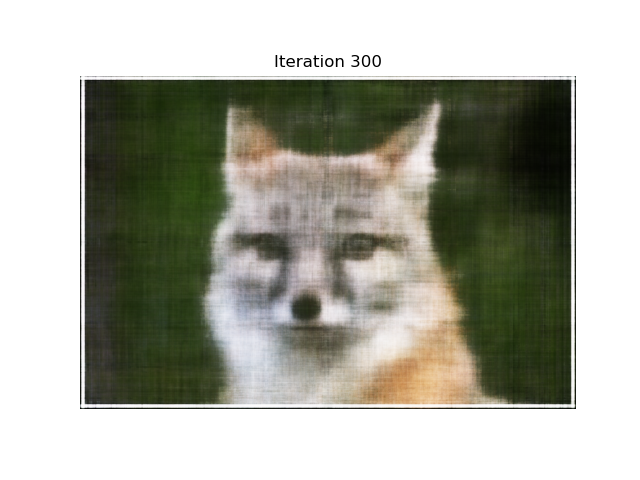
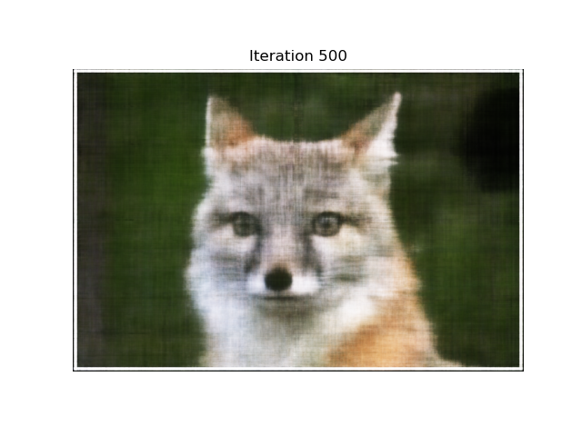
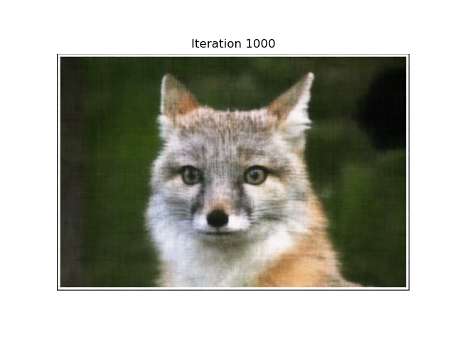
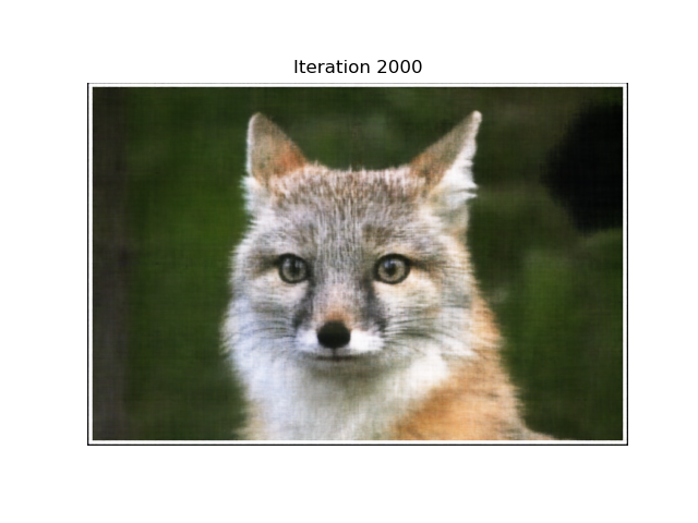
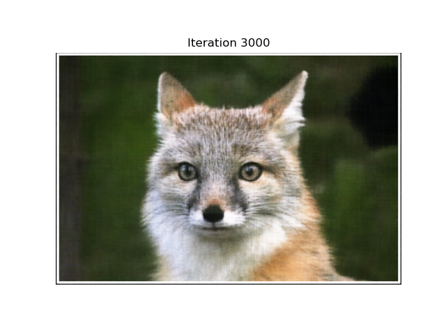
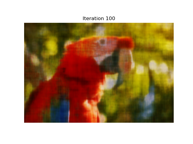
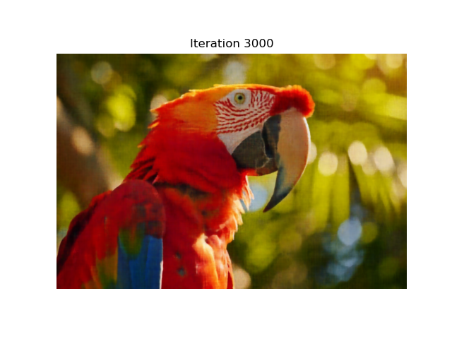
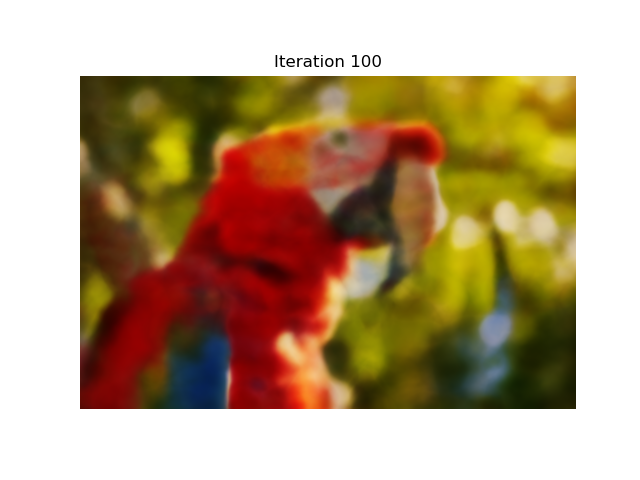
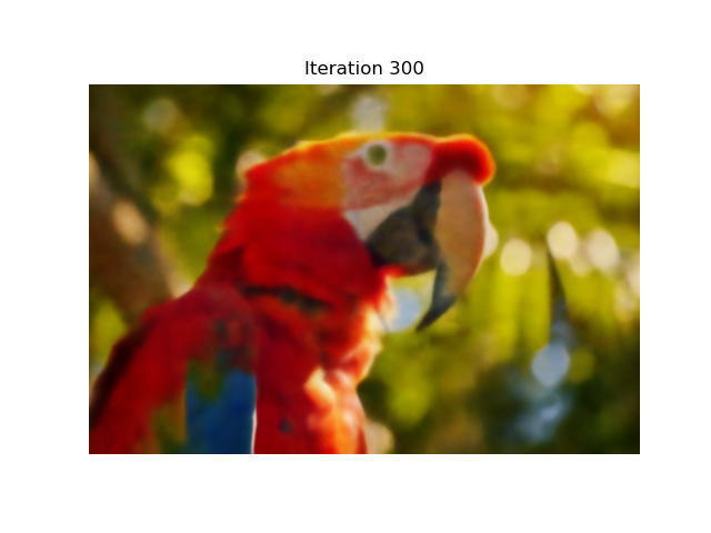
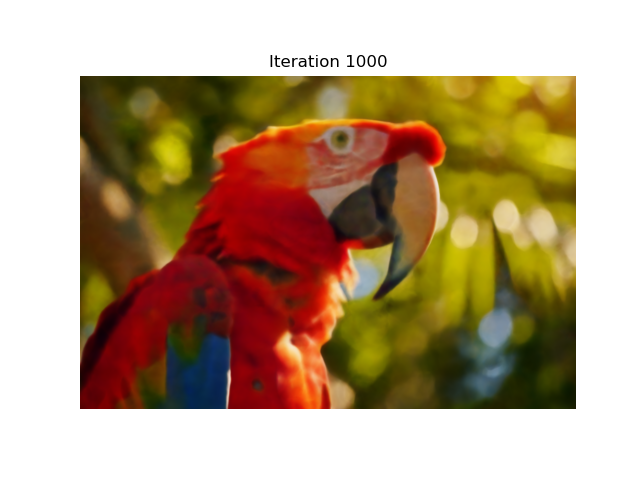
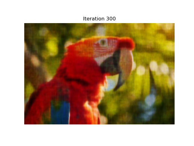
The training was run for a total of 3,000 iterations. Below are the predicted images at different stages of training for two different input images, illustrating how the model gradually learns to reconstruct each image:
Image 1: Fox

Iteration 100

Iteration 300

Iteration 500

Iteration 1000

Iteration 2000

Iteration 3000
Image 2: Parrot

Iteration 100

Iteration 300

Iteration 500

Iteration 1000

Iteration 2000

Iteration 3000
As shown in the images above, the network's predictions become progressively more accurate for both images, capturing finer details as training continues.
Hyperparameter Experiments
We experimented with different hyperparameters such as the number of layers, and positional encoding frequency \(L\). The following results show how these variations impact the model's performance. For each configuration, we display the predicted images at iterations 100, 1000, and 3000, along with the PSNR curve.
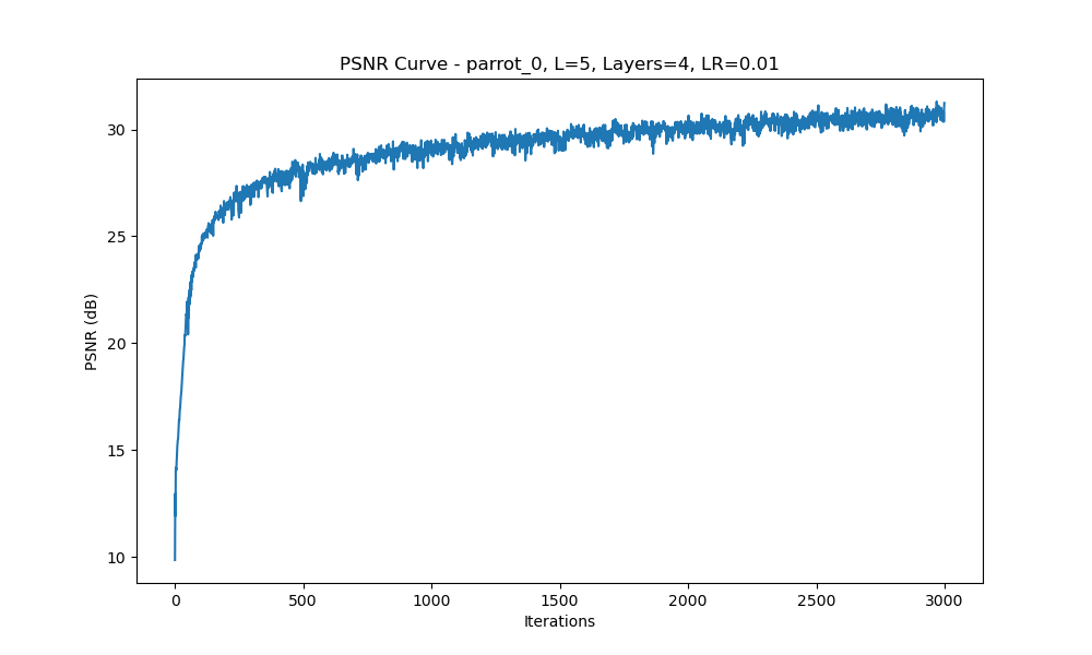
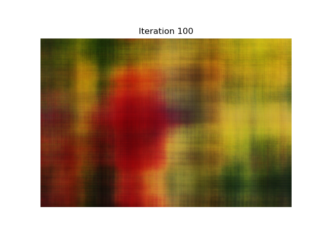
Configuration 1: Varying \(L\) Values (\(L = 5, 10, 15\)), 4 Layers, Learning Rate = 1e-2

Iteration 100

Iteration 300

Iteration 1000

Iteration 3000

PSNR Curve

Iteration 100

Iteration 300

Iteration 1000

Iteration 3000

PSNR Curve

Iteration 100

Iteration 300

Iteration 1000

Iteration 3000

PSNR Curve
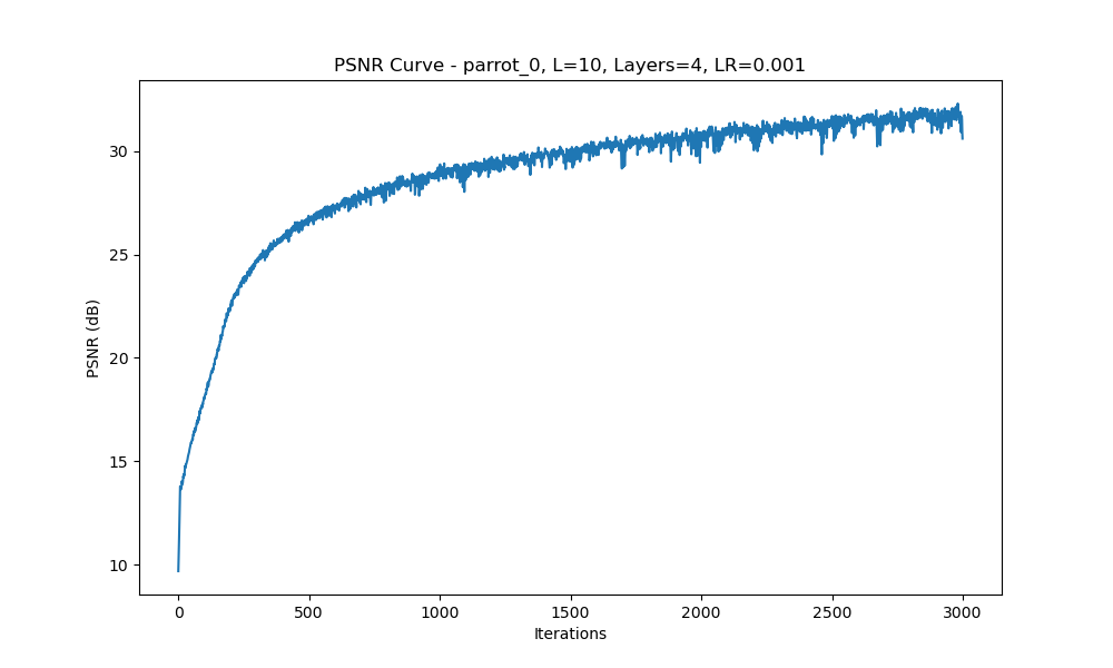
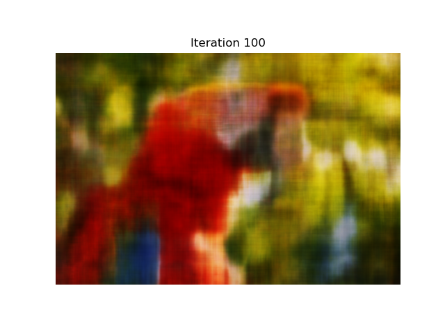
Configuration 2: Varying learning rate. (\(L = 10\)), 4 Layers, Learning Rate = 1e-2, 1e-3, 4e-3

Iteration 100

Iteration 300

Iteration 1000

Iteration 3000

PSNR Curve

Iteration 100

Iteration 300

Iteration 1000

Iteration 3000

PSNR Curve

Iteration 100

Iteration 300

Iteration 1000

Iteration 3000

PSNR Curve
Part 2: Fit a Neural Radiance Field from Multi-view Images
2.1: Create Rays from Cameras
Camera to World Coordinate Conversion
The transformation between the world space \( \mathbf{X_w} = (x_w, y_w, z_w) \) and the camera space \( \mathbf{X_c} = (x_c, y_c, z_c) \) can be expressed using a rotation matrix \( \mathbf{R_{3 \times 3}} \) and a translation vector \( \mathbf{t} \):
\[
\mathbf{X_c} = \begin{bmatrix} x_c \\ y_c \\ z_c \\ 1 \end{bmatrix} = \begin{bmatrix} \mathbf{R_{3 \times 3}} & \mathbf{t} \\ \mathbf{0_{1 \times 3}} & 1 \end{bmatrix} \begin{bmatrix} x_w \\ y_w \\ z_w \\ 1 \end{bmatrix}
\]
The inverse of this matrix, called the camera-to-world (c2w) transformation matrix, converts points from camera space to world space:
\[
\mathbf{X_w} = \text{c2w} \cdot \begin{bmatrix} x_c \\ y_c \\ z_c \\ 1 \end{bmatrix}
\]
Pixel to Camera Coordinate Conversion
To convert a pixel coordinate \( (u, v) \) to a point in the camera coordinate system \( \mathbf{x_c} \), we use the intrinsic matrix \( \mathbf{K} \):
\[
\mathbf{K} = \begin{bmatrix} f_x & 0 & o_x \\ 0 & f_y & o_y \\ 0 & 0 & 1 \end{bmatrix}
\]
The intrinsic matrix projects a 3D point \( (x_c, y_c, z_c) \) in the camera coordinate system to a 2D pixel coordinate \( (u, v) \):
\[
s \begin{bmatrix} u \\ v \\ 1 \end{bmatrix} = \mathbf{K} \begin{bmatrix} x_c \\ y_c \\ z_c \end{bmatrix}
\]
To invert this process and transform a pixel back to camera coordinates:
\[
\mathbf{x_c} = s \cdot \mathbf{K}^{-1} \begin{bmatrix} u \\ v \\ 1 \end{bmatrix}
\]
Pixel to Ray Conversion
A ray can be defined by an origin \( \mathbf{r_o} \) and a direction \( \mathbf{r_d} \). For a given pixel \( (u, v) \), the ray origin is the camera position:
\[
\mathbf{r_o} = \mathbf{c2w}_{[:3, 3]}
\]
To compute the ray direction \( \mathbf{r_d} \), convert the pixel to camera coordinates \( \mathbf{x_c} \), transform it to world coordinates \( \mathbf{x_w} \), and normalize:
\[
\mathbf{r_d} = \frac{\mathbf{x_w} - \mathbf{r_o}}{\|\mathbf{x_w} - \mathbf{r_o}\|}
\]
2.2: Sampling Rays and Points
To train the NeRF model, we need to sample points along the rays. The depth values \( t \) are uniformly sampled within a range \([near, far]\):
\[
t = \text{linspace}(near, far, n\_samples)
\]
The 3D points along each ray can be computed as:
\[
\mathbf{x} = \mathbf{r_o} + t \cdot \mathbf{r_d}
\]
To improve generalization and avoid overfitting, small perturbations can be added to the sampled points during training:
\[
t = t + \text{random\_perturbation}
\]
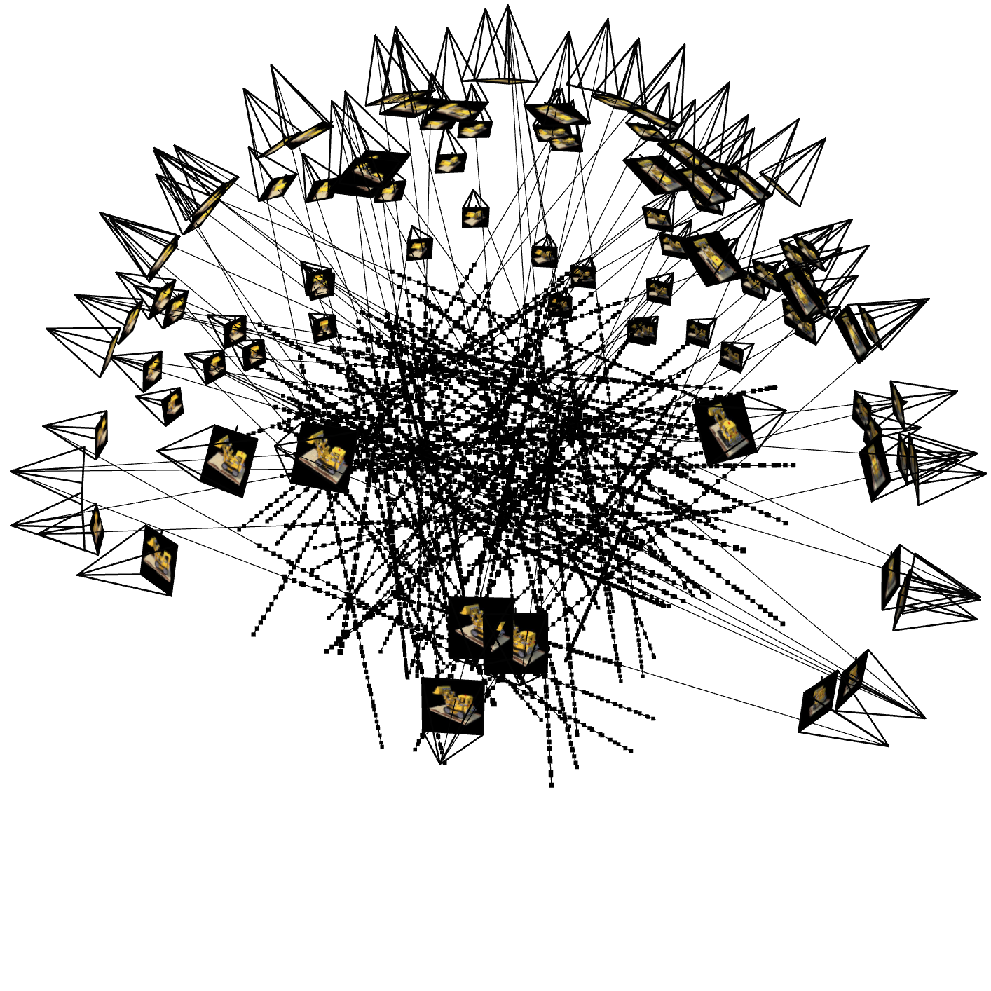
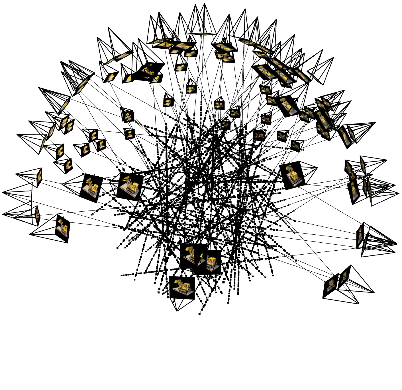
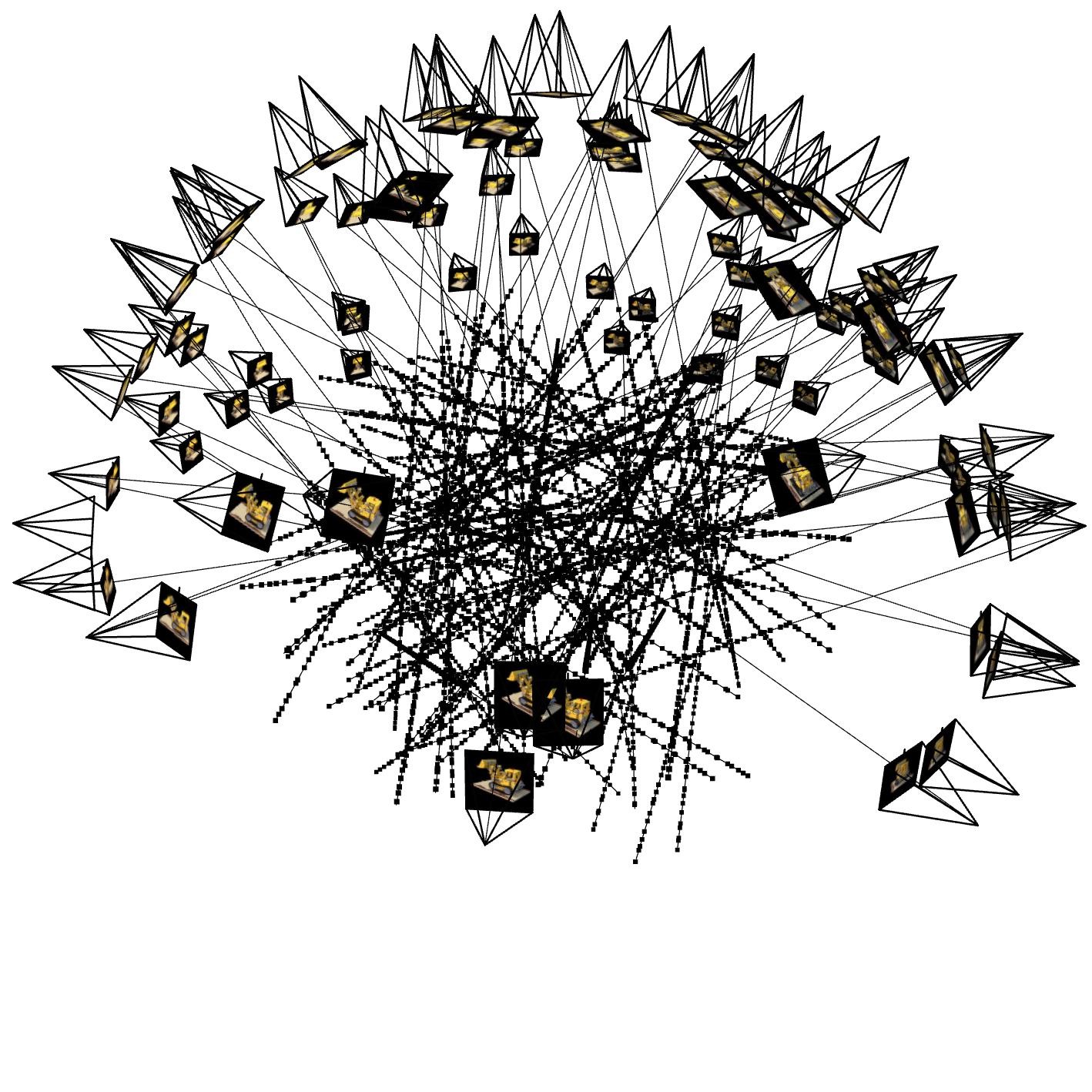
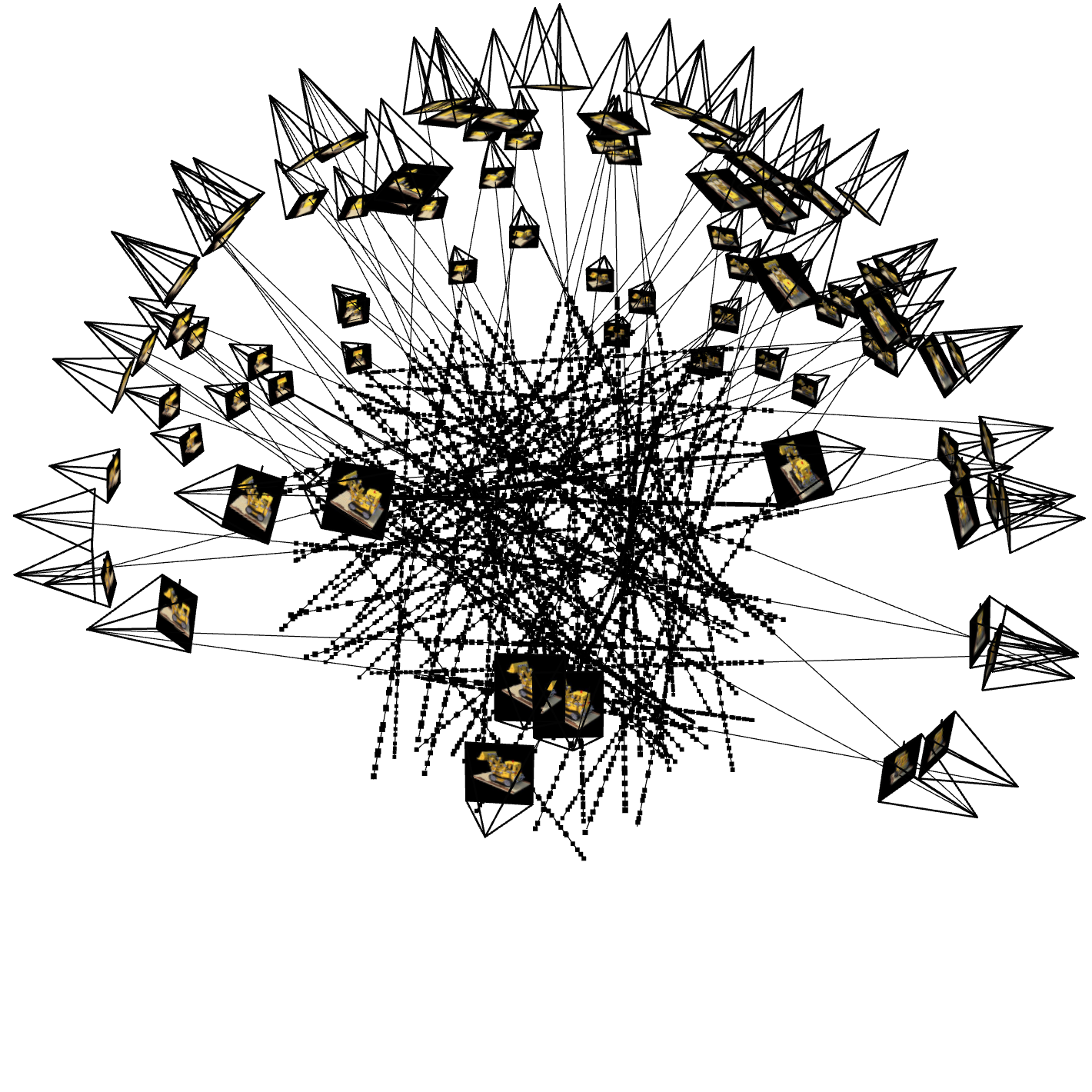
2.3: Visualization of Cameras, Rays, and Samples
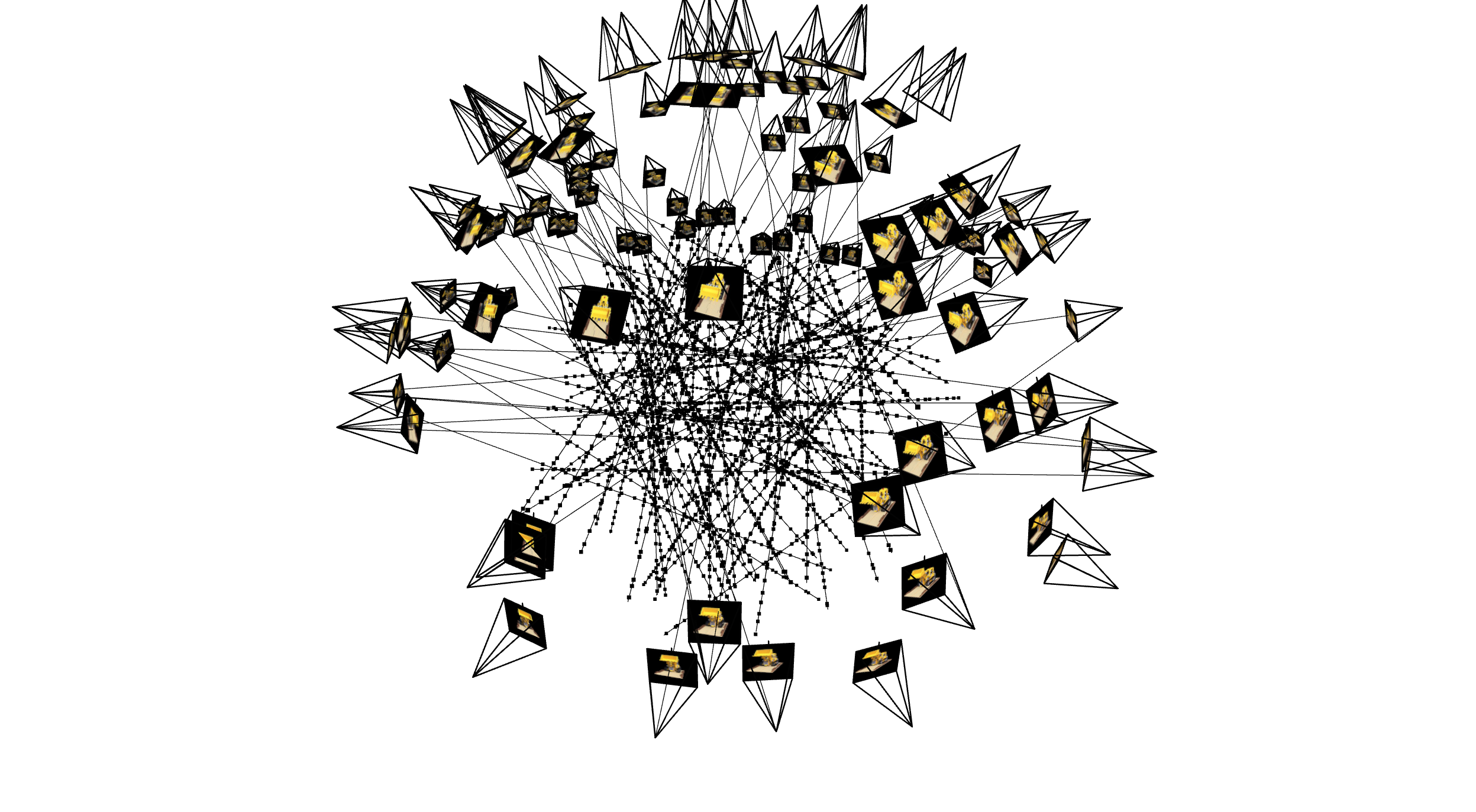
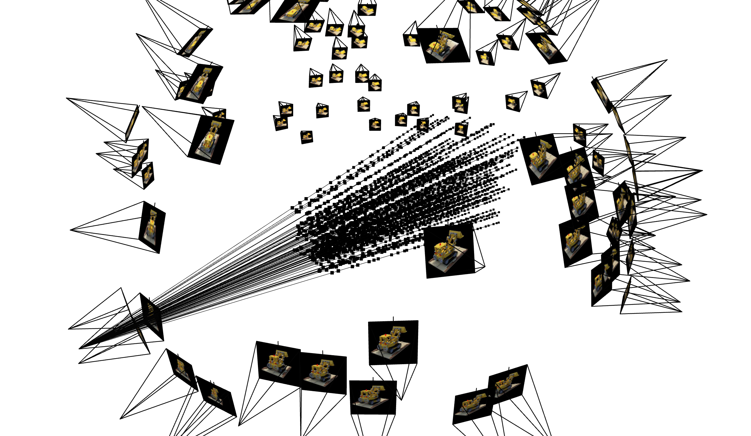
Below is a visualization showing the cameras, the rays emitted from the cameras, and the sampled points along those rays.

Figure 1: Visualization of Cameras, Rays, and Samples in 3D

Figure 1: Visualization of Cameras, Rays, and Samples in 3D
2.4: Neural Radiance Field
After sampling points in 3D, the goal is to predict the density and color of each point using a neural network. The network architecture is similar to the one used in Part 1, but with the following changes:
- Input: The network takes 3D world coordinates and a 3D ray direction vector as input.
- Deeper MLP: The network is deeper to handle the complexity of representing a 3D scene.
- Mid-layer Injection: The positional encoding (PE) of the input is injected into the middle layers of the MLP to help the network retain spatial information.
Network Architecture
The network first processes the positional encoding (PE) of the 3D input coordinates through several linear layers with ReLU activations. After a skip connection, the view direction (also encoded with PE) is concatenated with the features and passed through additional layers to produce the final RGB color and density outputs.

Figure: NeRF Network Architecture
This architecture allows the network to learn the 3D structure and color of the scene from multiple views.
2.5: Volume Rendering
The goal of volume rendering is to compute the final color of each ray by integrating the densities and colors predicted by the network along the ray's path. The core volume rendering equation is given by:
\[
C(\mathbf{r}) = \int_{t_n}^{t_f} T(t) \sigma(\mathbf{r}(t)) c(\mathbf{r}(t), \mathbf{d}) dt
\]
where \( T(t) = \exp\left(-\int_{t_n}^{t} \sigma(\mathbf{r}(s)) ds\right) \) is the probability that the ray has not been terminated before \( t \).
Discrete Approximation
To compute this integral numerically, we discretize it into a sum over sampled points along the ray. The discrete approximation is:
\[
\hat{C}(\mathbf{r}) = \sum_{i=1}^{N} T_i \left(1 - \exp(-\sigma_i \delta_i)\right) c_i, \quad \text{where} \quad T_i = \exp\left(-\sum_{j=1}^{i-1} \sigma_j \delta_j\right)
\]
Here, \( c_i \) is the color predicted by the network at the \( i \)-th sample point, \( \sigma_i \) is the density, and \( \delta_i \) is the distance between adjacent sample points.
Implementation Description
The implementation involves:
- Sampling Points: Uniformly sample points along each ray between a near and far range.
- Predicting Densities and Colors: Use the NeRF network to predict densities \( \sigma \) and colors \( c \) for the sampled points.
- Computing Weights: Calculate the transmittance \( T_i \) and weights based on the densities.
- Rendering: Sum the weighted colors to obtain the final rendered color for each ray.
This method allows us to render realistic images of the 3D scene by combining the contributions of all sampled points along each ray.
1. Visualization of Rays and Samples
The following figures show the visualization of the rays, samples, and camera frustums. These visualizations help verify that the rays are correctly generated from the camera positions.

Rays for Iter 50

Rays for Iter 100

Rays for Iter 200

Rays for Iter 500

Rays for Iter 800

Rays for Iter 1000
2. Training Process Visualization
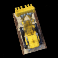
Below are the predicted images at different stages of training, illustrating how the network learns to reconstruct the 3D scene:

Iteration 50

Iteration 100

Iteration 200

Iteration 500

Iteration 800

Iteration 1000
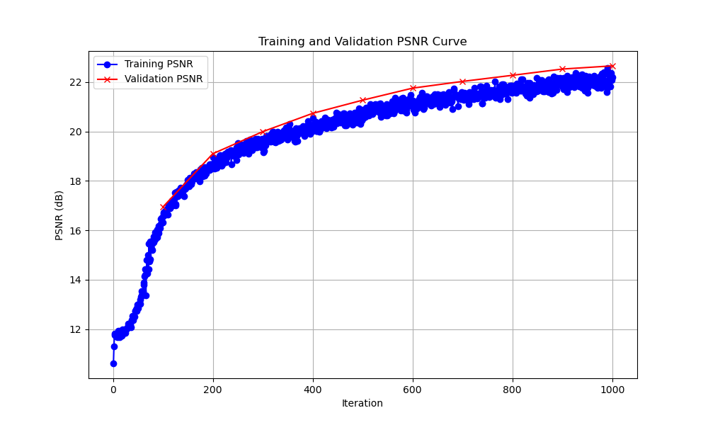
3. PSNR Curve on the Validation Set
The PSNR curve shows the reconstruction quality on the validation set across iterations. PSNR of 23.16 is achieved

Figure: PSNR Curve on Validation Set
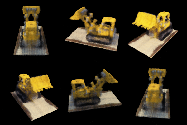
4. Novel View Rendering
The trained NeRF can render novel views of the Lego scene from unseen camera angles. The following video demonstrates the rendered views using the test camera poses:

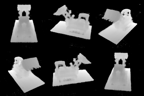
Depth Map Visualization - Novel Views
5. Depth Map Video
The depth map visualization helps understand the geometry of the scene. This feature is part of the Bells and Whistles, enhancing the visualization of depth maps. Below is a video showing the depth maps with contrast enhancement:

Depth Map Visualization
Z

