Filters & Frequencies: Edges, Hybrid Images, and Blending
Working in the frequency domain to extract edges, create hybrid images that change meaning with viewing distance, and blend images seamlessly via Laplacian pyramids. Ends with the famous 'oraple.'
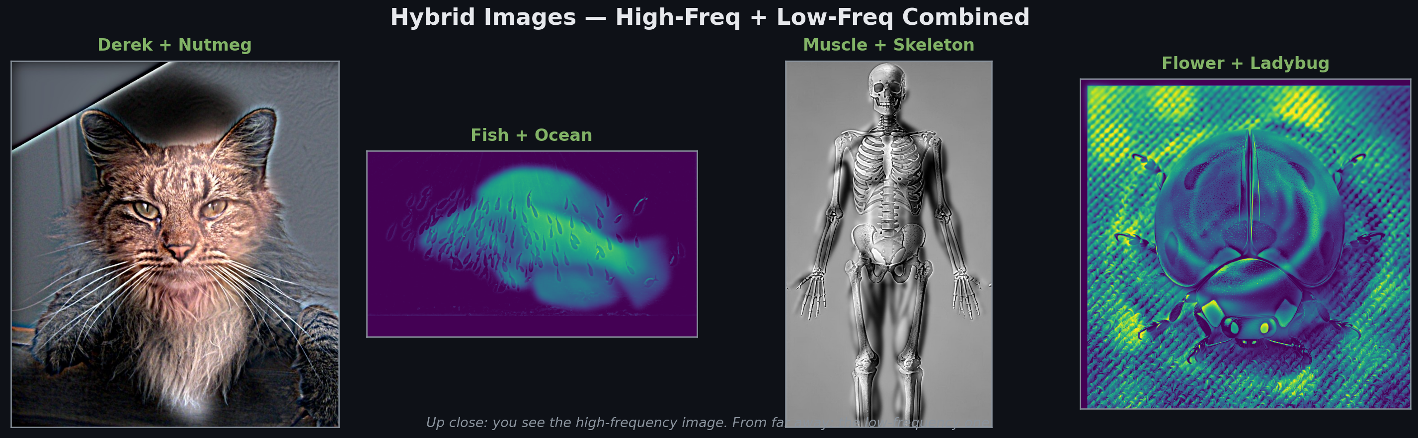
Most of classical image processing is frequency analysis in disguise. Edge detection is a high-pass filter. Sharpening adds back high frequencies. Hybrid images combine one image’s high frequencies with another’s low frequencies; your visual system resolves the ambiguity based on viewing distance. Seamless blending works by splitting images into frequency bands, blending each band separately, then reconstructing.
Edge Detection
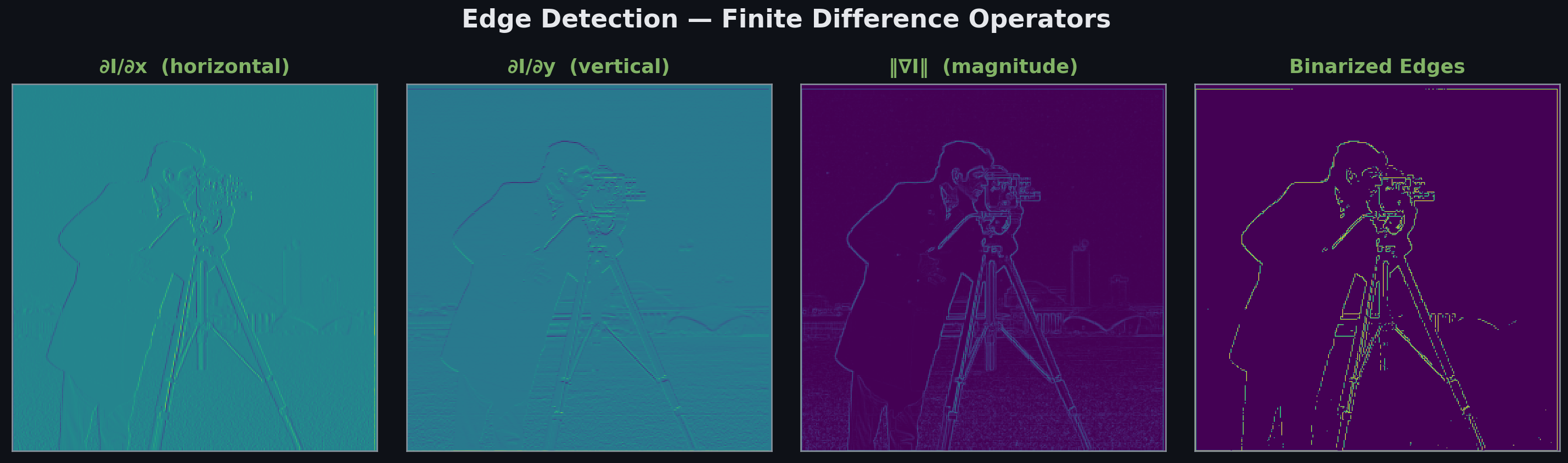
Edges appear where image intensity changes rapidly. The partial derivative in x is approximated with a finite difference kernel , and similarly for y. The gradient magnitude is:
The problem with differentiating noisy images directly: differentiation amplifies high-frequency noise, turning a single noisy pixel into a sharp spike in the derivative. The fix is the Derivative-of-Gaussian (DoG) filter: convolve the Gaussian with the difference kernel first, then apply that single filter to the image:
Convolution is associative, so computing once and applying it produces identical results to smoothing then differentiating, with one fewer convolution pass. The Gaussian suppresses noise at scales below before the derivative sees it.
Unsharp Masking
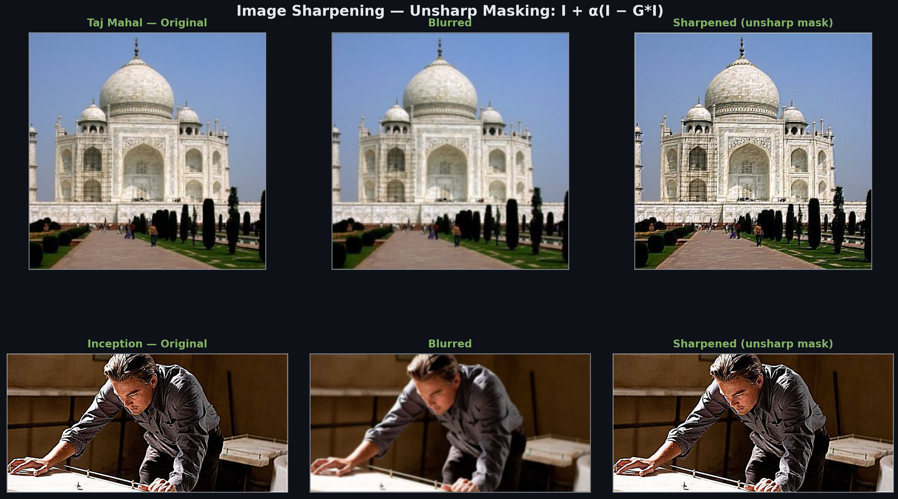
Sharpening amplifies edges without changing overall brightness. The low-frequency content of an image is ; subtracting it from the original isolates high frequencies . Adding those back scaled by gives the unsharp mask formula:
Rearranging: , a single combined filter. The result exaggerates edges, which the visual system reads as increased sharpness even though no new information was added. Over-sharpening ( too large) produces visible ringing artifacts (Gibbs phenomenon) around sharp edges.
Hybrid Images
Look at the flower-ladybug image in the hero: up close you see the ladybug’s high-frequency detail; from a distance the flower’s low-frequency shape dominates. The construction:
and set the cutoff frequency. The choice of which image contributes low vs high frequencies determines what you see close vs far. The human visual system’s spatial frequency sensitivity drops sharply above about 6 cycles/degree, so at distance, only the low-frequency image is visible. The two frequency bands occupy non-overlapping parts of the spectrum and don’t interfere with each other.
Alignment of the two images at the semantic level (eyes to eyes, faces at same scale) is critical; misaligned anchors produce jarring hybrids.
Multiresolution Blending
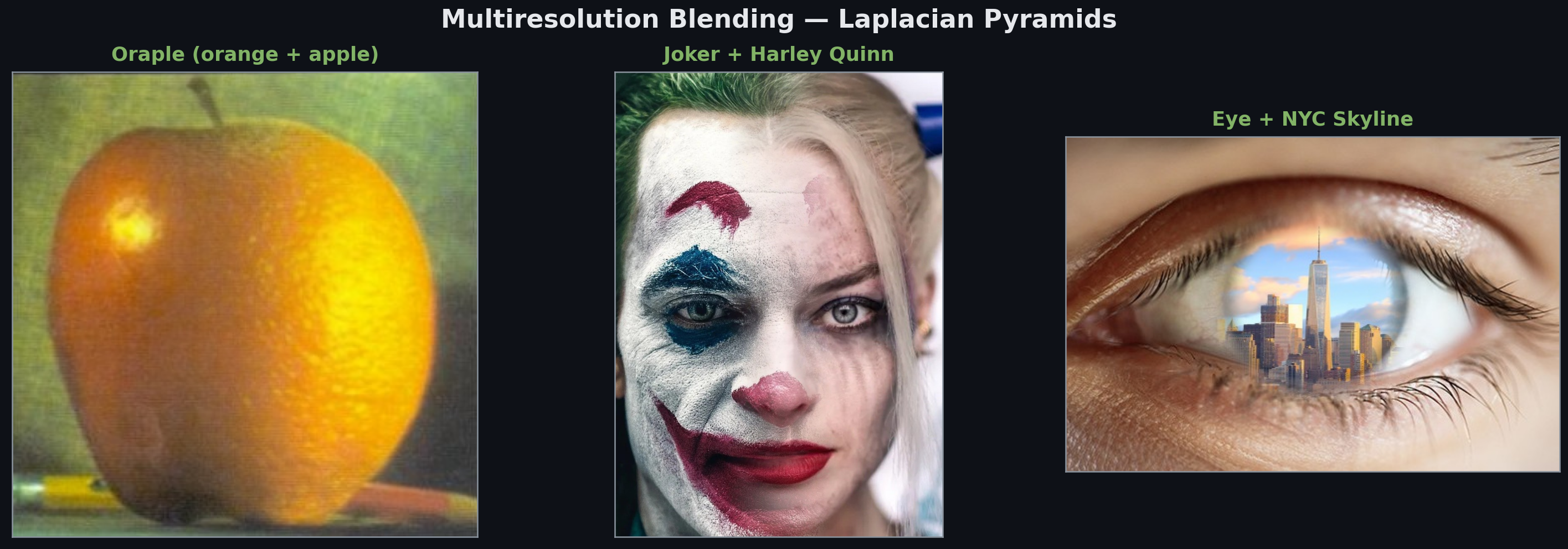
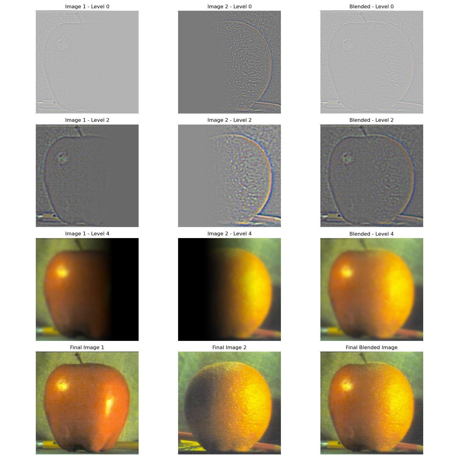
Naive alpha-blending at a seam leaves a visible transition because high-frequency mismatches (sharp edges) are blended with the same soft transition used for low-frequency color differences. The fix: blend each frequency band independently with a mask appropriate to that band’s scale.
The Laplacian pyramid decomposes an image into frequency bands. Let be the -th level of a Gaussian pyramid (each level downsampled by 2× from the previous). The Laplacian level is:
Each captures a band of frequencies centered around the Nyquist frequency of level . To blend:
- Build Laplacian pyramids , for both images
- Build a Gaussian pyramid from the mask
- Blend each level:
- Reconstruct by summing upsampled levels
At high-frequency levels, the mask is crisp (sharp cut between left and right). At low-frequency levels, the mask has been blurred many times, so the color transition is gradual. The right panel above shows pyramid levels 0, 2, and 4 for the oraple: high frequencies are cut sharply at the seam; low frequencies blend smoothly across the whole image.
Related projects
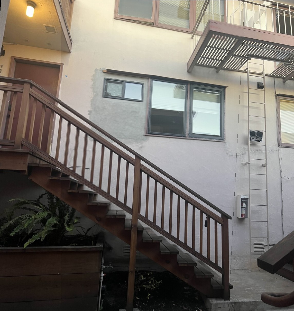
Auto-Stitching Photo Mosaics
Building a panorama pipeline from scratch: Harris corner detection, Adaptive Non-Maximal Suppression, feature matching, RANSAC for homography estimation, and Laplacian-pyramid blending.
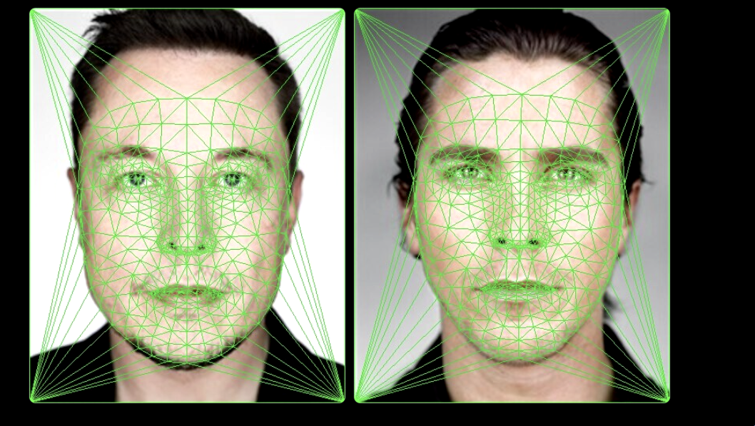
Face Morphing with Delaunay Triangulation
Smooth warping between two faces via point correspondences, Delaunay triangulation, and affine warps per triangle. Plus: population mean faces and caricature generation by extrapolation.
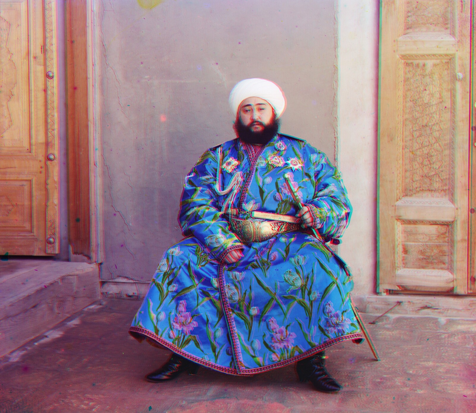
Colorizing 1907 Russian Empire Photographs
Reconstructing color from Sergei Prokudin-Gorskii's glass plate negatives (captured 1907–1915) using image pyramids and normalized cross-correlation alignment.