Auto-Stitching Photo Mosaics
Building a panorama pipeline from scratch: Harris corner detection, Adaptive Non-Maximal Suppression, feature matching, RANSAC for homography estimation, and Laplacian-pyramid blending.
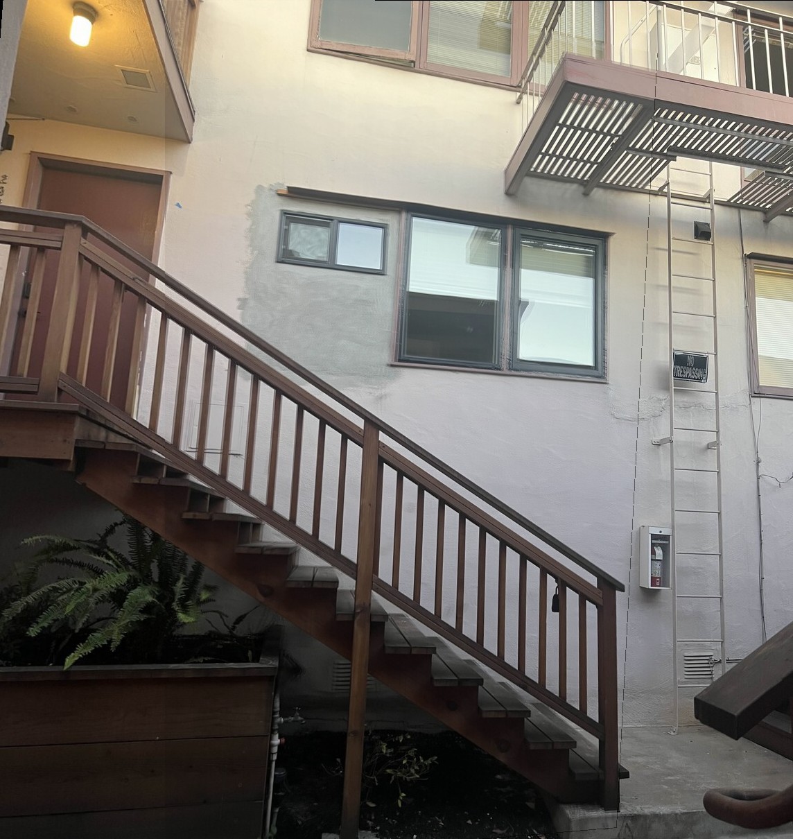
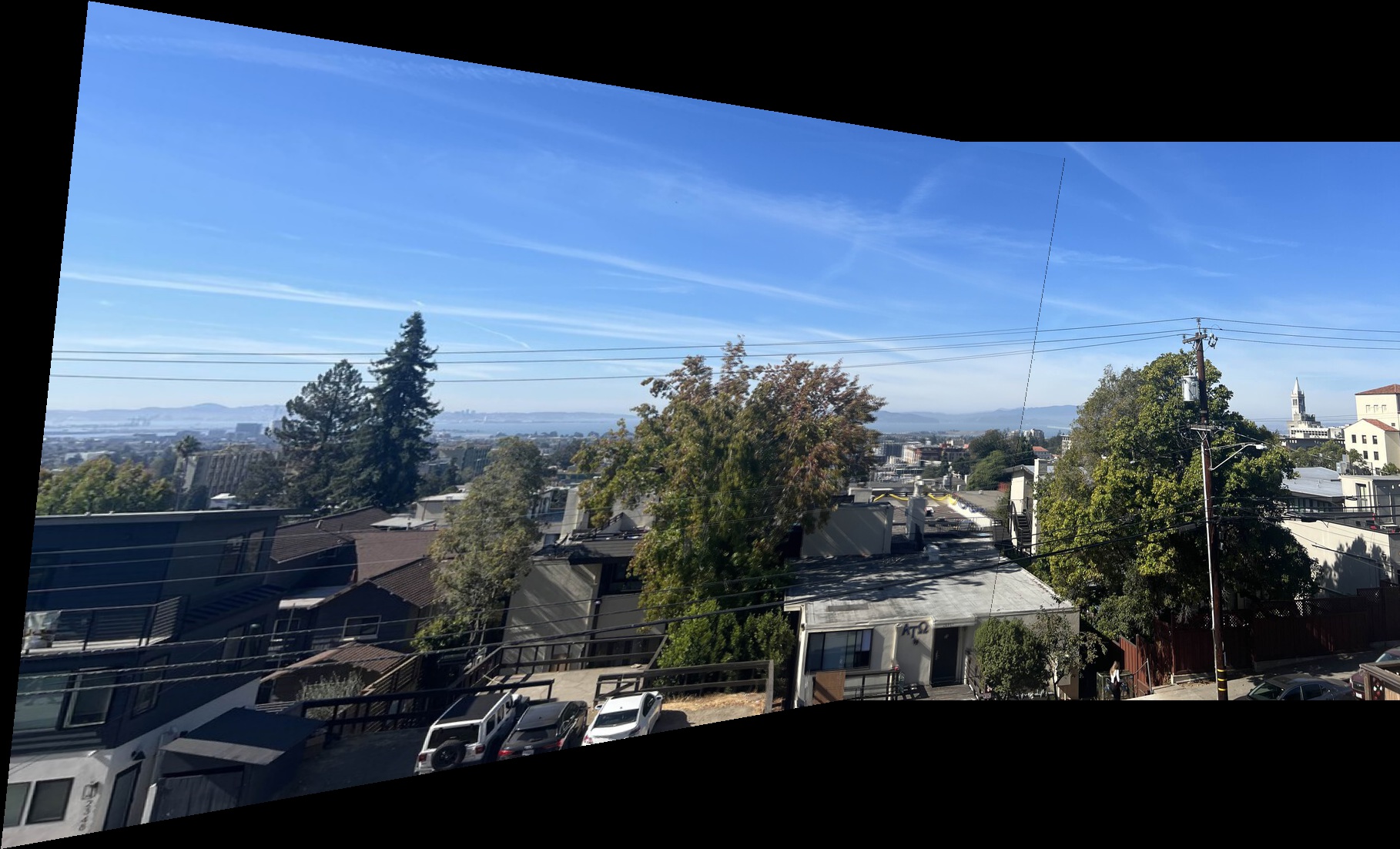
Taking two overlapping photos and producing a seamless panorama is a cascade of five hard problems: finding distinctive points, distributing them evenly, matching them across views, filtering bad matches robustly, and blending without seams. Each step uses well-established CV techniques; composing them end-to-end is where it gets interesting.
Harris Corners and ANMS
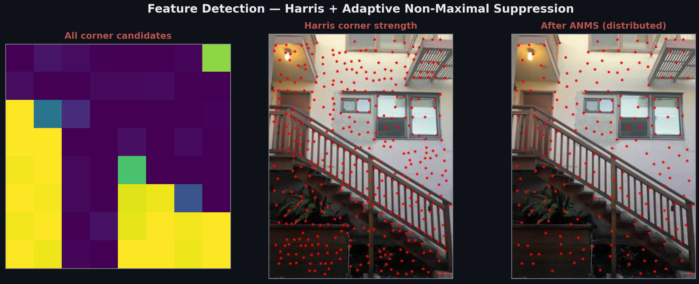
The Harris corner response measures how much the image changes when you shift a window in any direction:
where are image gradients computed over the window. indicates a corner (both eigenvalues large), an edge (one large eigenvalue), a flat region.
Raw Harris over-detects: textured regions produce dense clusters of high- points while sparse areas get nothing. ANMS fixes this by enforcing spatial spread: a corner at position is suppressed unless it is the strongest corner within radius , where is its suppression radius. Keeping the top- corners by yields a spatially uniform distribution, which matters for matching: uniformly distributed features constrain the homography better than clustered ones.
Feature Descriptors and Matching
Each surviving corner gets a descriptor: sample a 40×40 patch around it, downsample to 8×8, normalize to zero mean and unit variance (bias/gain normalization). Normalization makes descriptors invariant to local brightness and contrast changes; the same surface lit differently will match.
Matching: for each descriptor in image A, find the two nearest neighbors in image B (by SSD). Accept the match only if:
Lowe’s ratio test rejects ambiguous matches: if the best match is nearly as good as the second-best, the feature is probably in a repeated-texture region and the match is unreliable. This eliminates most false positives cheaply, before RANSAC.
RANSAC Homography Estimation
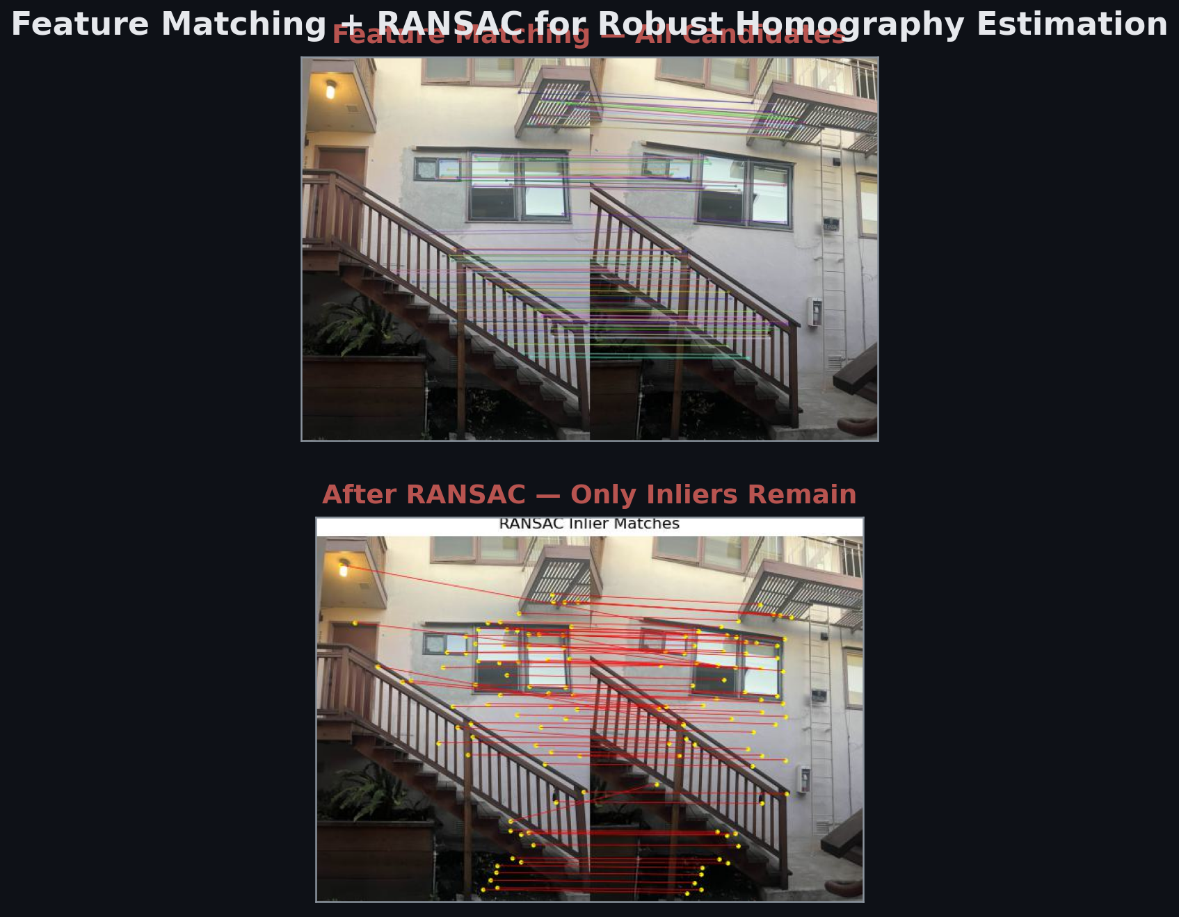
Even after the ratio test, outliers remain from repeated structures (railings, windows). RANSAC handles them:
- Sample 4 random point correspondences
- Solve for the homography using the Direct Linear Transform (DLT): stack the 4 point equations into and solve via SVD
- Count inliers: points where pixels
- Repeat 1000 times, keep the with the most inliers
- Refit using all inliers from the best iteration
The DLT for each point pair contributes two rows to :
With 4 points: 8×9 system, null space gives the 9 entries of (up to scale). The green lines above are the 1000-iteration RANSAC inliers; red matches were correctly rejected.
Warping and Blending
With in hand, warp image A into image B’s coordinate frame using inverse warping. For each output pixel, apply to find the source coordinate, then bilinear-interpolate. Forward warping would leave holes; inverse warping doesn’t.
The overlap region is blended with a Laplacian pyramid: construct the pyramid for each warped image, blend each level using a mask that ramps linearly across the overlap, reconstruct. This makes the seam invisible because color transitions happen gradually at low frequencies while sharp detail is composited cleanly at high frequencies.
Results
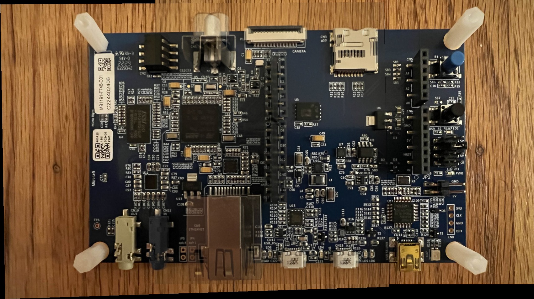
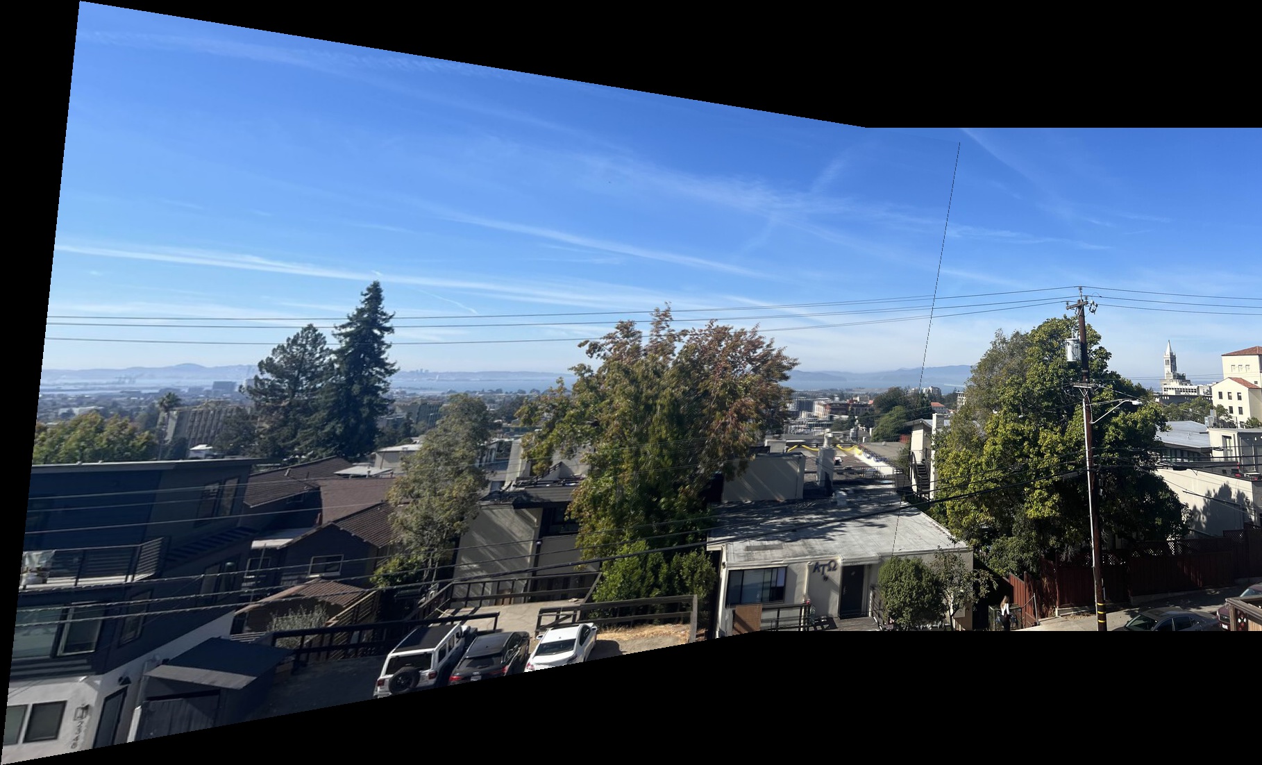
The pipeline succeeds across very different scene types: architectural geometry (ladder/exterior), fine electronic detail (PCB), and indoor scenes. Failure modes: scenes with insufficient overlap, scenes where all features lie in a plane (degenerate homography), and scenes with moving objects in the overlap region (RANSAC can’t recover a consistent when the scene itself changes between frames).
Why the Pipeline Composes
Each stage absorbs noise from the previous. Harris over-detects, so ANMS filters spatially. Matching over-connects, so the ratio test filters ambiguous pairs. The ratio test leaves outliers, so RANSAC filters geometrically inconsistent ones. The pipeline is deliberately redundant: classical CV survives individual component failures because each stage imposes an independent constraint, and errors have to defeat all of them simultaneously.
Related projects
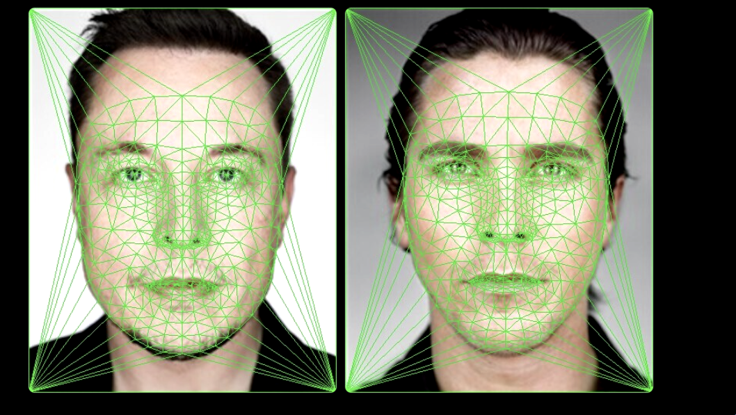
Face Morphing with Delaunay Triangulation
Smooth warping between two faces via point correspondences, Delaunay triangulation, and affine warps per triangle. Plus: population mean faces and caricature generation by extrapolation.
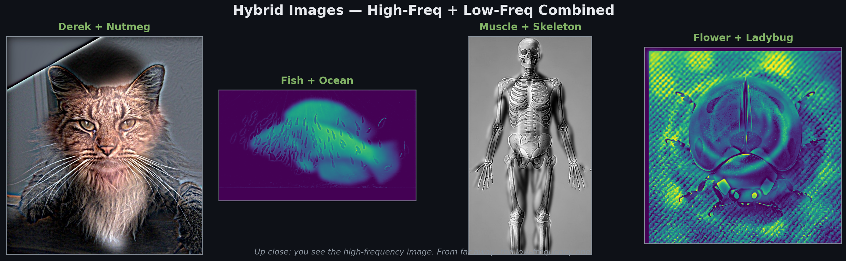
Filters & Frequencies: Edges, Hybrid Images, and Blending
Working in the frequency domain to extract edges, create hybrid images that change meaning with viewing distance, and blend images seamlessly via Laplacian pyramids. Ends with the famous 'oraple.'
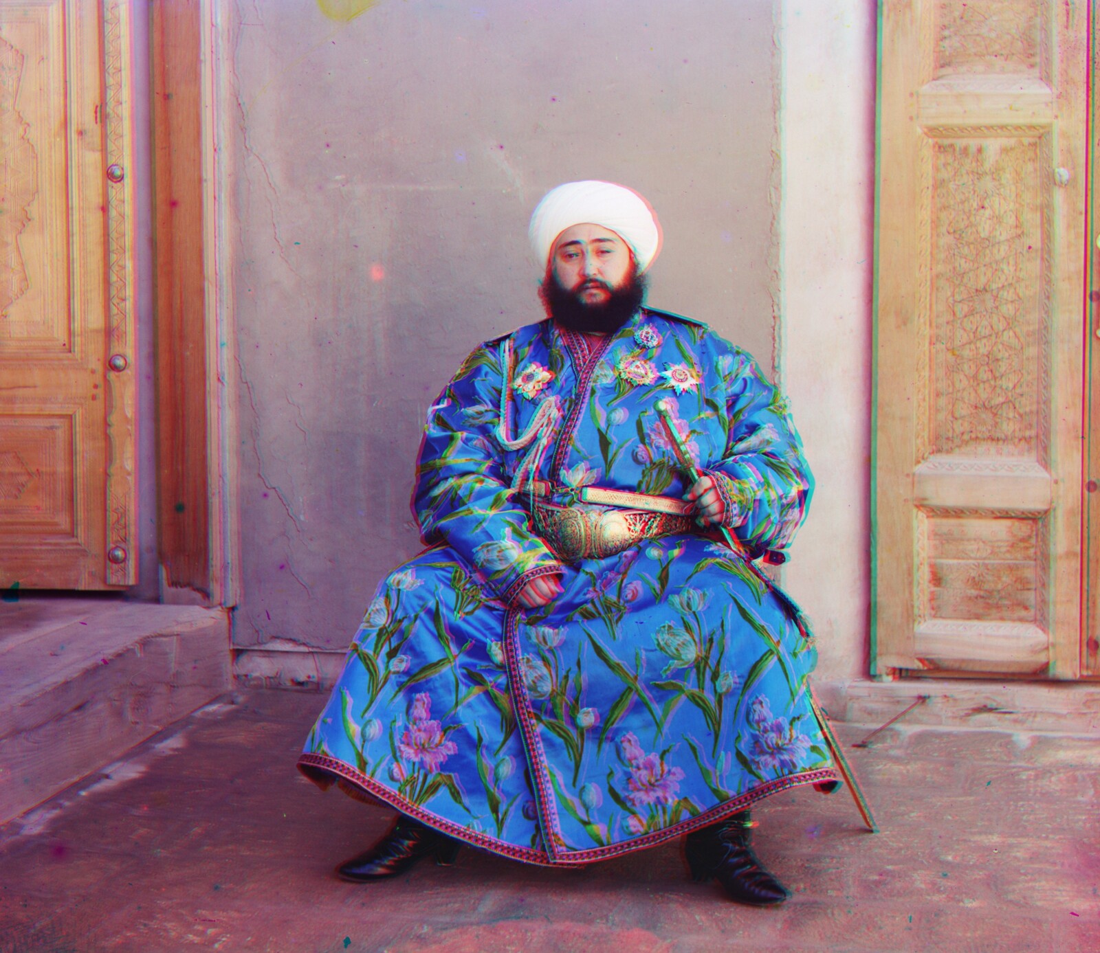
Colorizing 1907 Russian Empire Photographs
Reconstructing color from Sergei Prokudin-Gorskii's glass plate negatives (captured 1907–1915) using image pyramids and normalized cross-correlation alignment.