Nonlinear MPC for Autonomous Racing
Progress-maximizing NMPC for a full-scale Dallara AV-24 competing in the Indy Autonomous Challenge. Two-timescale architecture: a full-lap minimum-time NLP solved offline with a double-track Pacejka vehicle model produces the Track Trajectory Library, while an NMPC at 100 Hz in a Frenet frame executes it with RTI. Validated in AWSIM (best lap 117.6 s, 207 km/h max) and on the physical car.
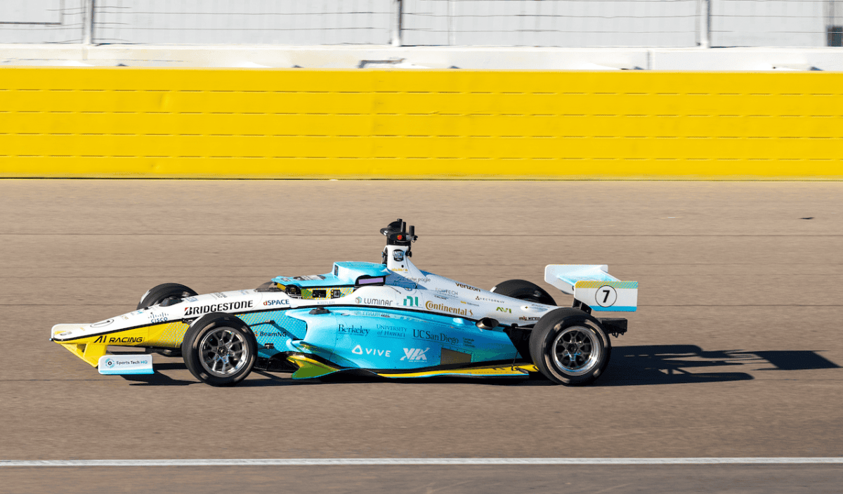
The Indy Autonomous Challenge is a head-to-head autonomous racing competition where full-scale Dallara AV-24 open-wheel race cars compete at circuits like Indianapolis Motor Speedway, reaching speeds above 180 mph (290 km/h). No human in the loop. This capstone report describes a ground-up redesign of UC Berkeley’s IAC controller, a Nonlinear MPC that abandons reference-tracking in favor of directly maximizing forward progress. My contribution is Chapter 2: the offline trajectory optimization layer that defines the global racing strategy the online controller executes.
The Two-Timescale Architecture
A controller running at competition speeds faces two problems that operate on incompatible timescales. Planning (deciding where to brake, which line to take through a corner sequence, how to trade exit speed from one turn against entry speed into the next) requires global reasoning over the entire 3.5 km circuit. Execution (rejecting disturbances, compensating for estimation error, staying dynamically feasible) must happen within the 10 ms budget of a single control cycle. No real-time solver can do both.
The solution is a clean separation: a full-lap minimum-time NLP solved offline (before the race, no time limit) produces the Track Trajectory Library (TTL) encoding the optimal racing strategy. An NMPC running online at 100 Hz receives the TTL as its task specification and focuses entirely on tracking it under real-world mismatch. The offline layer says what the car should do over the lap. The online controller figures out how to actually do it.
Chapter 2: Offline Trajectory Optimization
The Minimum-Time Problem
The continuous-time minimum-lap-time problem is straightforward to write down:
The periodicity constraint enforces a closed lap. To solve it numerically, the track centerline is discretized into segments of arc length . The free final time is replaced by per-segment time intervals , each a decision variable. The discretized cost is:
The first term is the lap time, the dominant objective. The control-effort and control-rate regularization terms (with small weights) prevent numerically degenerate bang-bang solutions that the real car cannot follow.
Track boundary constraints keep lateral deviation within the drivable area with non-uniform safety margins; the optimizer uses more of the available width on high-speed straights and tightens margins through the most dangerous sections:
The resulting NLP has roughly 15,000 decision variables across nodes. Solving it is what takes minutes, which is perfectly acceptable for an offline computation.
Double-Track Vehicle Model
| Feature | Offline double-track | Online bicycle |
|---|---|---|
| Tire patches | 4 independent | 2 axles |
| Tire model | Pacejka Magic Formula (post-peak) | Soft linear saturation |
| Wheel load transfer | Explicit per-wheel | Axle-averaged |
| Aerodynamics | Full downforce + drag | Omitted |
| States | 6 + load dynamics | 6 |
| Solve time | Minutes | <10 ms |
The offline model represents all four tire contact patches independently, capturing effects the online bicycle model averages away:
- Individual wheel loads. Longitudinal and lateral load transfer resolve per wheel. Under hard braking into a left-hander, the right-front tire carries the largest normal load and therefore the most available grip; the double-track model represents this asymmetry directly.
- Pacejka Magic Formula. Each tire’s forces are computed from the full Magic Formula with load-dependent stiffness coefficients (, , , ), capturing the full nonlinear slip-force curve including the post-peak region where force declines with increasing slip.
- Road surface coupling. Banking and grade vary along the track and affect both effective normal load and lateral force balance. At Laguna Seca’s Corkscrew, these effects contribute up to 40% of the vertical loads.
The per-wheel friction constraint is the friction ellipse applied independently to each corner:
Equilibrium-based wheel dynamics. A naive double-track model adds four wheel-spin states to the NLP, making it stiff and much larger. Instead, we use an equilibrium formulation: the slip ratio is solved quasi-statically from the torque command at each node, eliminating the four states. This makes the NLP tractable without sacrificing the friction coupling.
B-Spline Track Representation
Raw surveyed GPS coordinates of inner and outer barriers are converted into ENU frame, then fitted with cubic B-splines using a smoothing parameter that balances fidelity to the survey points against geometric smoothness. The spline representation gives analytic derivatives of curvature, banking, and grade at arbitrary arc-length positions, critical for CasADi’s automatic differentiation.
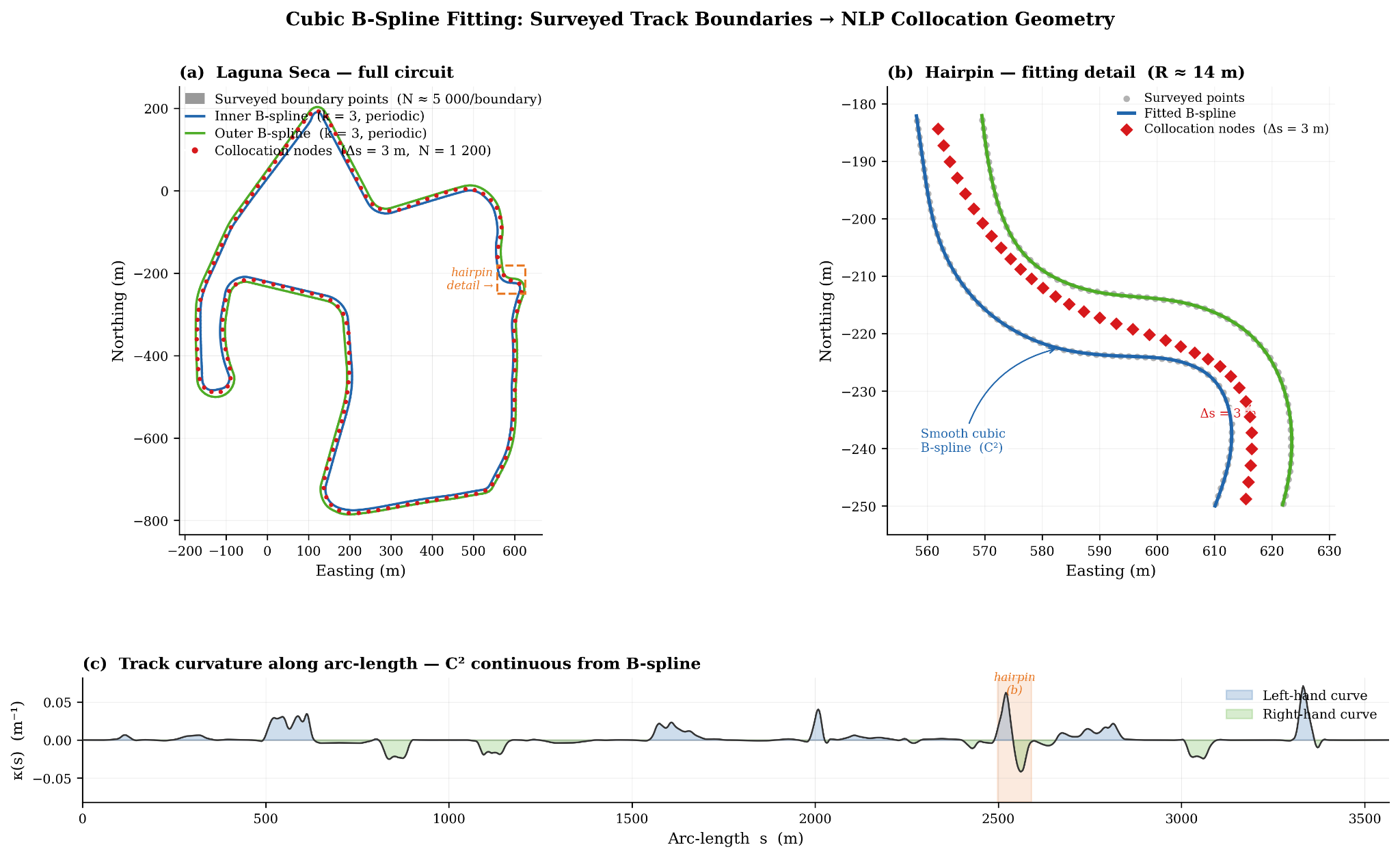
The centerline is re-sampled at uniform arc-length intervals () to define the NLP’s collocation grid. At each node, boundary distances and , curvature , banking , and grade are evaluated from the splines and passed as fixed parameters. The C² continuity from cubic B-splines ensures the curvature profile (bottom panel) is smooth, essential for a well-posed NLP.
CasADi + IPOPT
The NLP is constructed symbolically in CasADi, which provides automatic differentiation of the cost and all constraints. This generates exact gradients, Jacobians, and Hessians. No finite-difference approximation. This matters especially for Pacejka expressions: nested nonlinearities like the Magic Formula evaluated at load-dependent slip values are poorly served by finite differences.
The assembled NLP is solved by IPOPT (Interior Point OPTimizer), a primal-dual interior-point method. Configuration:
- Convergence tolerance , constraint-violation tolerance
- Cold start (from QSS init): ~200 iterations, ~200 s
- Warm start (previous solution): ~50–90 iterations, ~50 s
A bug we found and fixed. The warm-start control scaling was being double-applied: applied once in Python when building the warm-start guess and again inside the CasADi/IPOPT interface. This caused IPOPT to enter the restoration phase on every solve, an expensive fallback for infeasible iterates. After fixing the double-application, warm-start performance improved by ~50× (200 s → ~50 s).
Sensitivity analysis on Laguna Seca lap time (v3 → v4 solver configuration):
| Parameter change | Lap time improvement |
|---|---|
| Friction coefficient: 1.1 → 1.25 | −4.4 s |
| Track margins: 1.5 m → 0.3 m | −2.3 s |
| Steering rate weight : 0.75 → 0.3 s | −0.3 s |
| Regularization weights: 25× reduction | −1.1 s |
QSS initialization. Before handing the NLP to IPOPT, a quasi-steady-state forward simulation propagates the vehicle model along the centerline, computing the maximum speed at each point under steady-state cornering assumptions. The result is dynamically plausible but suboptimal, a feasible warm start that keeps IPOPT out of the restoration phase from the first iteration.
Track Geometry and the Optimal Speed Profile
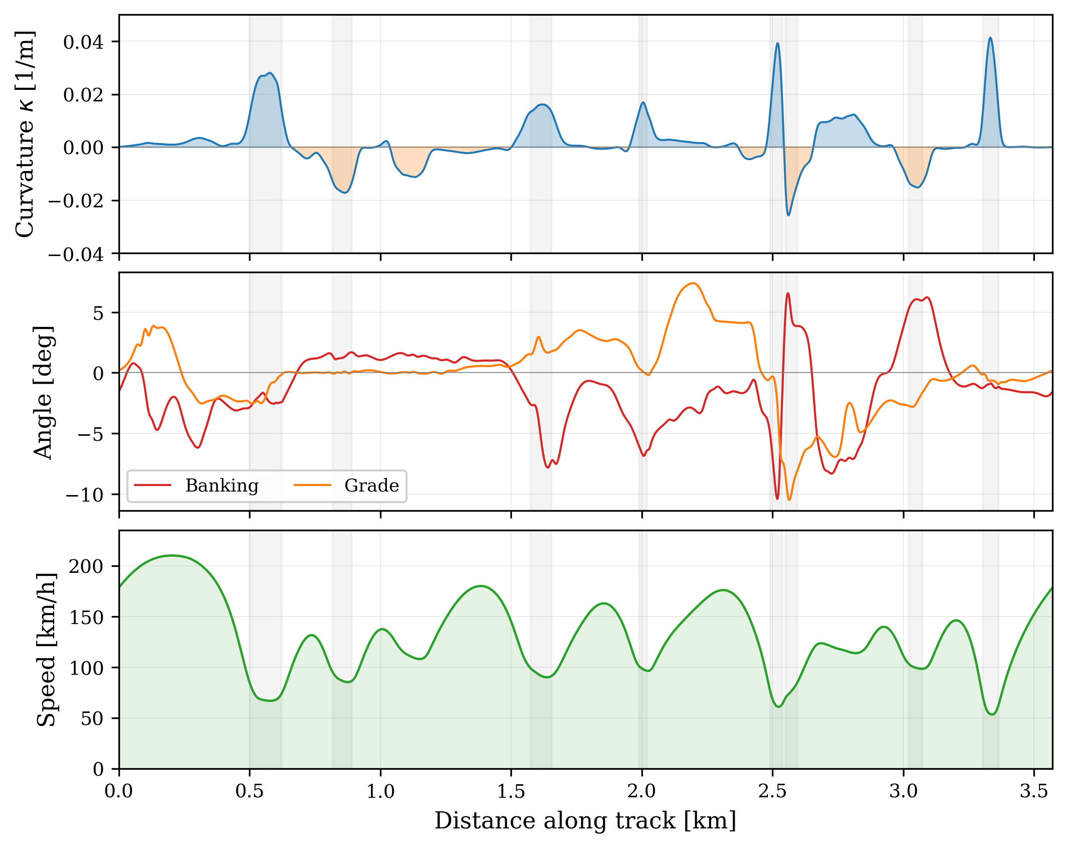
Top panel: signed curvature , distinguishing left and right turns. Middle panel: road banking and grade from survey data; the dramatic feature around 2.5 km is the Corkscrew. Bottom panel: the optimized speed profile. It is strongly anti-correlated with curvature, reflecting the globally coordinated braking strategy. The optimizer doesn’t just slow down for each corner independently; it adjusts exit speed from one corner to set up entry into the next.
The Track Trajectory Library (TTL)
The optimizer’s solution is post-processed into a standardized CSV called the Track Trajectory Library (TTL), which serves as the interface contract between the offline and online layers:
| Field | Symbol | Role in online control |
|---|---|---|
| Position | Global racing line in ENU frame | |
| Heading | Track-tangent direction | |
| Arc-length progress | Trajectory indexing and Frenet projection | |
| Reference speed | Longitudinal target for MPC cost | |
| Curvature | Feedforward steering demand | |
| Boundary positions | Track-limit constraints in MPC | |
| Banking angle | Normal load and lateral force correction | |
| Grade angle | Longitudinal gravitational component | |
| Nominal dynamic state | Warm-start context for MPC horizon |
In practice the team maintains a library of TTLs per track computed by running the same optimizer with different boundary-margin and lane-constraint settings:
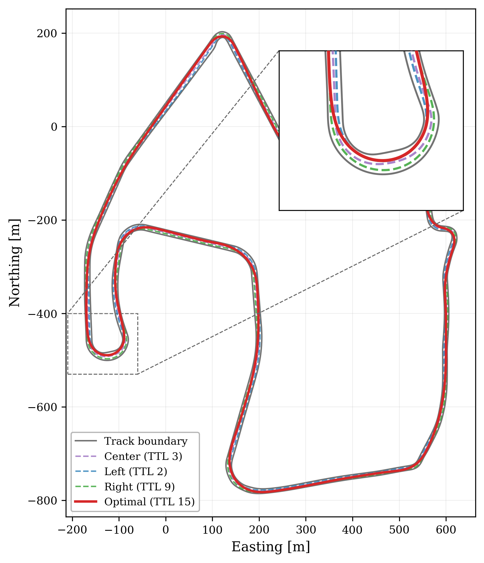
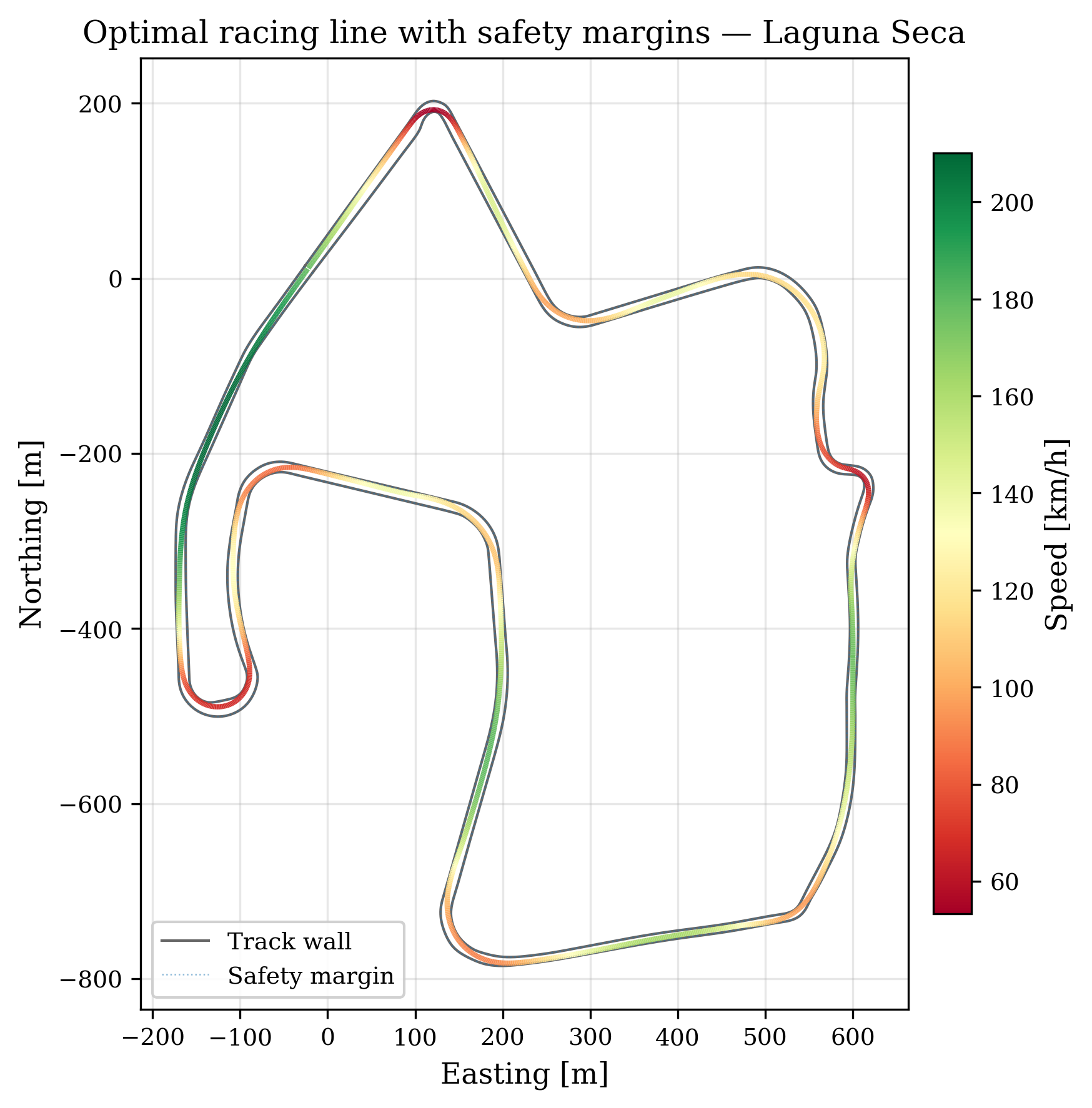
The hairpin inset (left) shows where the lines diverge most: the optimal trajectory (red) clips the apex more aggressively than the constrained variants, using available track width to carry higher cornering speed. The right figure color-codes the racing line by speed. At runtime the control stack selects TTLs by race situation: a pit stop command triggers a switch to TTL 27; an overtaking maneuver biases toward the left or right line.
Online NMPC Formulation
Progress-Maximizing Objective
The online NMPC operates in a curvilinear Frenet frame attached to the TTL racing line. Rather than tracking a precomputed speed schedule, it directly maximizes arc-length rate , the rate of advance along the track. This lets the solver simultaneously determine the optimal speed profile and lateral line within its prediction horizon, adapting to the current vehicle state instead of blindly following a plan.
The reference-tracking approach collapses the “what to do” and “how to do it” problems into one proxy objective. Progress-maximizing MPC separates them cleanly: the TTL defines a feasible corridor; the MPC optimizes freely inside it.
The stage cost at each discretization step :
The first term drives progress maximization. The remaining terms regularize by penalizing lateral deviation , heading error , steering effort , and torque magnitude. The terminal cost includes a velocity-maximizing term to avoid the horizon-end braking artifact in finite-horizon formulations.
Vehicle Models
Kinematic bicycle, 4-state :
where . Assumes no tire slip. Computationally cheap but limited at high lateral accelerations.
Dynamic bicycle, 6-state , adding body-frame velocities and yaw rate. The arc-length rate becomes:
Newton–Euler dynamics in the body frame:
Why the online model is simpler. A double-track model adds stiff ODE dynamics: body modes at ~5 Hz and tire dynamics at ~50 Hz create a 10× stiffness gap that forces small integration steps or implicit solvers, blowing the 10 ms budget. The bicycle model avoids this while still capturing the limit-handling physics that matter for the MPC’s prediction.
Tire Model: Combined-Slip with Friction Ellipse
The online controller uses a soft linear saturation model: smooth, symbolically differentiable, and capturing the essential friction coupling. Raw forces are linear in slip:
The combined force magnitude is saturated via hyperbolic tangent, enforcing a friction ellipse:
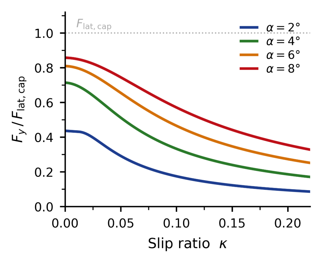
where . The chart above shows exactly why this coupling matters: at slip angle , applying even 0.05 slip ratio (light braking) cuts available lateral force from 81% to ~50% of capacity. The MPC must account for this trade-off when planning trail-braking entries. Without combined slip, it would over-predict available cornering grip during braking.
Additional model layers for fidelity:
- Aero model: downforce increases effective grip and drag at high speed
- Load transfer lag: eliminates unrealistic instantaneous weight transfer
- 3D road effects: banking and grade (Corkscrew: up to 40% of vertical loads):
- Tire moments: rolling resistance (~5% of longitudinal acceleration); aligning torque (pneumatic trail × lateral force, up to 50% of yaw moment)
Constraints
Hard constraints: Actuator box bounds. Front torque constrained to brake only (); rear torque spans braking to maximum propulsion.
Soft constraints with / slack penalties to preserve feasibility when the car is at the track limit:
- Track boundaries: Lateral deviation within with configurable safety margin; high penalty weight.
- Speed limit: Upper bound with penalty.
- Brake safety: Constraint preventing simultaneous front braking and rear acceleration, enforced with (not ) because the bilinear product has a zero Jacobian at the nominal operating point, violating LICQ.
Discretization
Direct multiple shooting over steps at 50 Hz (1-second lookahead), using a two-stage Runge–Kutta (Heun) integrator. The resulting NLP has approximately 450 decision variables plus slack variables.
Real-Time Execution
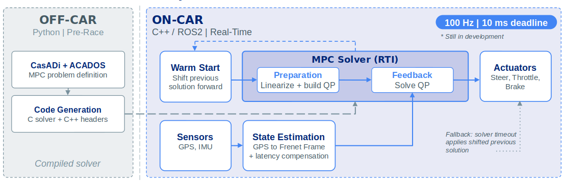
Real-Time Iteration (RTI) Split
The baseline controller solved the full NLP to convergence each cycle: unpredictable solve times, incompatible with a hard deadline. The redesign uses RTI:
- Preparation phase: linearize dynamics and build QP matrices using the warm-started solution from the previous cycle. This runs before the new sensor measurement arrives.
- Feedback phase: incorporate the latest state measurement and solve the single pre-built QP. Fast, bounded time.
Result: deterministic sub-10 ms actuation timing. The key insight is that between consecutive 10 ms control cycles, the optimal solution drifts only slightly; a warm-started single Newton step lands close to the new optimum.
The control loop is sensor-driven, not clock-driven: each new sensor measurement triggers exactly one Newton step. No measurement means no computation. This directly bounds worst-case latency to one iteration’s cost.
Conditioning the Single Newton Step
A single Newton step is only reliable if the QP is well-conditioned. Three layers:
- Variable scaling: bring all state and control variables to comparable magnitudes (). Without this, mixing 200 km/h velocities and 0.1 rad steering angles into one Hessian creates ill-conditioning.
- Eigenvalue-projection regularization: eigendecompose the Hessian and project flat directions up to a controlled minimum eigenvalue. This prevents the Newton step from blowing up along poorly-excited directions.
- Primal–dual warm-start: carry the primal solution, dual variables, and active-set information from the previous cycle. This keeps the next linearization close to the prior optimum and makes the single step sufficient.
Latency Compensation
Between sensor measurement and actuator command, 20–100 ms of transport delay elapses. At 200 km/h, even 50 ms of uncompensated delay is 2.8 m of unmodeled position error, significant relative to track width.
The state estimator compensates by forward-simulating the vehicle dynamics from the most recent GPS measurement through the history of actuator commands that have been issued but not yet reflected in sensor data:
The MPC plans from where the vehicle will be when the command takes effect, not from where it was when the measurement was captured.
Software Architecture
Offline (Python, pre-race)
generate.py
  ├── ModelSpec
  │     dynamics, cost, constraints
  ├── AbstractAcadosBuilder
  │     MpcAcadosBuilder
  │     StateEstimatorAcadosBuilder
  ├── CasADi symbolic expressions
  └── acados → C solver + C++ headers
Online (C++17, 100 Hz)
Pipeline<TModel>
  ├── AcadosStateEstimatorSolver
  │     GPS → Frenet + latency comp.
  ├── WarmStarter<TSolution>
  │     shift_solution() each cycle
  ├── AcadosMpcSolver (RTI)
  │     PREPARATION → FEEDBACK
  └── to_actuator_commands()
The central abstraction is Pipeline<TModel>, a C++17 template parameterized by vehicle model. The template bundles type aliases (State, Control, Solution, parameter vectors) and a Conversions class implementing AbstractConversions. Switching between kinematic and dynamic bicycle models is a single template argument change and a rebuild. No changes to the pipeline, ACADOS wrappers, or test suite.
The Python code generator outputs C++ header files with type-safe structs having a DIMENSION constant and static_assert enforcing standard-layout and size. Dimensional mismatches between the generated solver and runtime code are caught at compile time.
ROS2 integration is deliberately thin: the MpcNode handles only message conversion and lifecycle management, delegating all control logic to the model-agnostic pipeline. A thin bridge node decouples the MPC from the rest of the autonomy stack (localization, planner, vehicle interface); the bridge translates between the two ROS namespaces without adding any safety-critical logic.
Test Suite: 25,900 Lines of Tests
| Layer | Description |
|---|---|
| Unit tests | Bicycle dynamics, tire models, cost/constraint Jacobians, generated struct layout, ACADOS compatibility, powertrain conversion, actuator safety filters |
| Pipeline tests | Cross-validate Python acados solver output against C++ runtime (pybind11 bindings); closed-loop lap completion on synthetic and real track geometries |
| dSPACE VEOS | Software-in-the-loop with full vehicle dynamics before on-car authority |
| Ghost controller | Run alongside the existing controller on-car, publish telemetry, without actuating |
| Track testing | Closed-loop validation at speed on the physical car |
The codebase: ~7,800 lines of production code, ~5,100 lines of comments, ~25,900 lines of tests, a 3.3× test-to-code ratio. TDD enables aggressive refactoring: the architecture underwent several major iterations (kinematic → dynamic bicycle, parameter pipeline restructuring) with full confidence from the test safety net.
The pybind11 pipeline tests deserve special mention: they expose the C++ runtime to Python for direct numerical comparison against the reference Python solver. This catches bugs that only appear when symbolic expressions are compiled and run, invisible in unit tests of individual components.
Validation
AI-Assisted Development
The project integrates Claude Code into the development workflow under project-level llm.md and style_guide.md instructions. The AI assistant operates under the same TDD discipline as human developers: every feature begins with a failing test. This workflow offloads boilerplate generation, refactoring, and configuration propagation while TDD guards against the primary risk of AI-generated code: plausible-looking but incorrect implementations.
Ghost Controller: On-Car Without Actuation
Before giving the new controller authority over the physical car, we ran it in ghost mode alongside the existing controller on the actual Dallara AV-24: consuming live sensor data and publishing command telemetry, but not actuating. This validated the full software stack under real sensor noise and timing without any safety risk.
| Ghost controller metric | Value |
|---|---|
| Diagnostics publish rate | 24.5 Hz |
| MPC actuation topic rate | 20.2 Hz |
| Solve time (p95) | 24.9 ms |
| Healthy solves | 75.6% |
| Fallback (shifted prev. solution) used | 3.4% |
The p95 solve time of 24.9 ms is from the full NLP IPOPT solver. The RTI two-phase split (preparation + feedback) reduces the latency-critical feedback phase to a single QP solve, achieving the sub-10 ms deadline.
Closed-Loop Pipeline Test
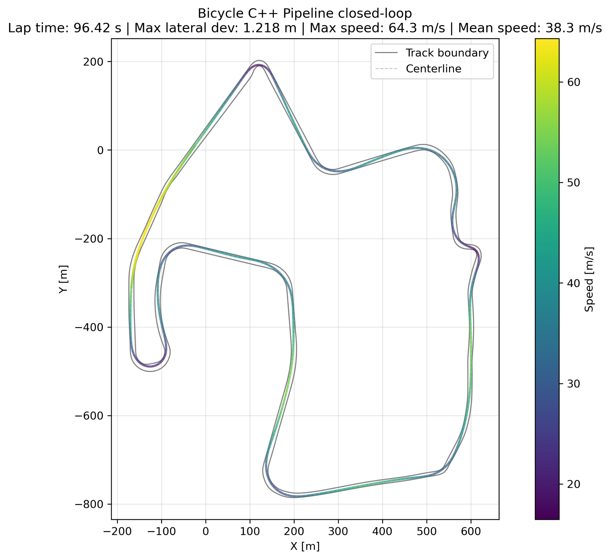
The C++ pipeline integration test runs the complete MPC stack (state estimation → warm start → solve → actuator commands) in closed loop against the bicycle dynamics model. Best lap: 96.42 s, max speed 64.3 m/s (231 km/h), max lateral deviation 1.218 m. The trajectory closely tracks the optimal racing line (shown in the figure), demonstrating that the full stack, from GPS input to actuator command, behaves correctly end-to-end.
AWSIM Simulation at Laguna Seca
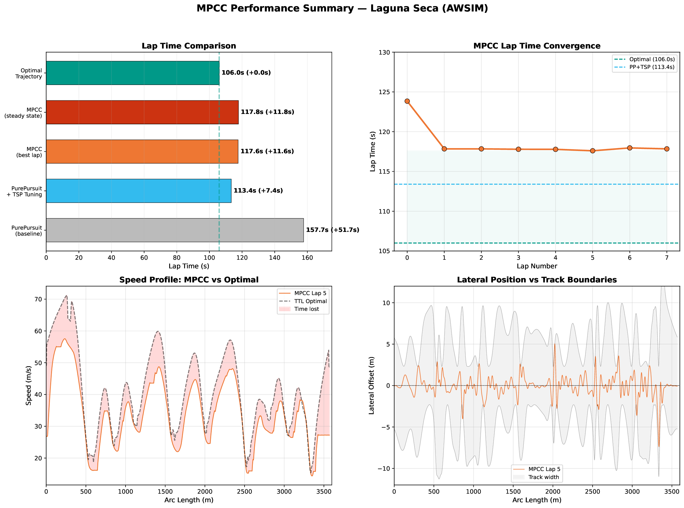
AWSIM validation on the full Laguna Seca circuit (3.5 km):
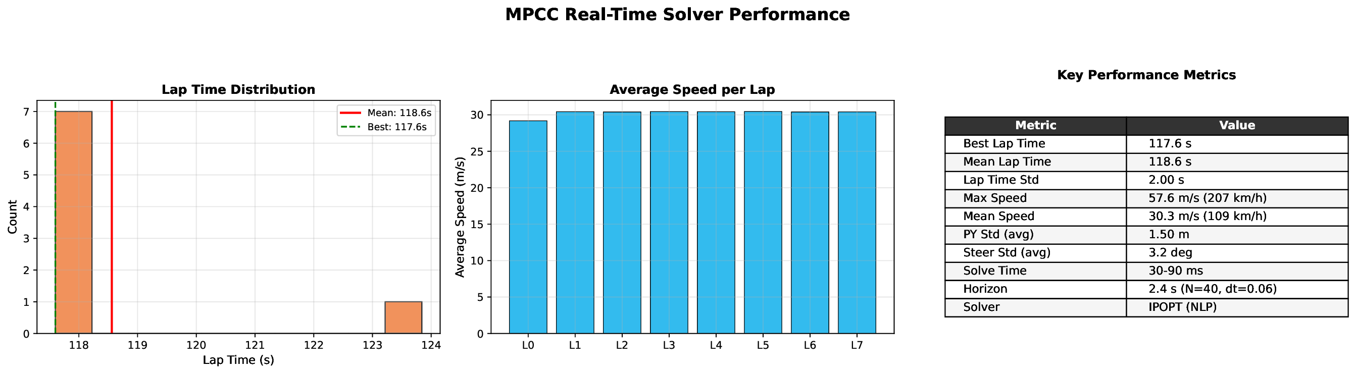
| Metric | NMPC (MPCC) | PurePursuit baseline | PurePursuit + TSP | Theoretical optimal |
|---|---|---|---|---|
| Best lap time | 117.6 s | 157.7 s | 113.4 s | 106.0 s |
| Max speed | 207 km/h | N/A | N/A | N/A |
| Mean speed | 109 km/h | N/A | N/A | N/A |
| Lateral std (avg) | 1.50 m | N/A | N/A | N/A |
| Lap time std | 2.0 s | N/A | N/A | N/A |
The NMPC is 25% faster than the PurePursuit baseline and within 11% of the theoretical optimal. The PurePursuit + TSP variant (113.4 s) requires a hand-tuned speed profile for this specific track; the NMPC requires no such tuning and generalizes across tracks.
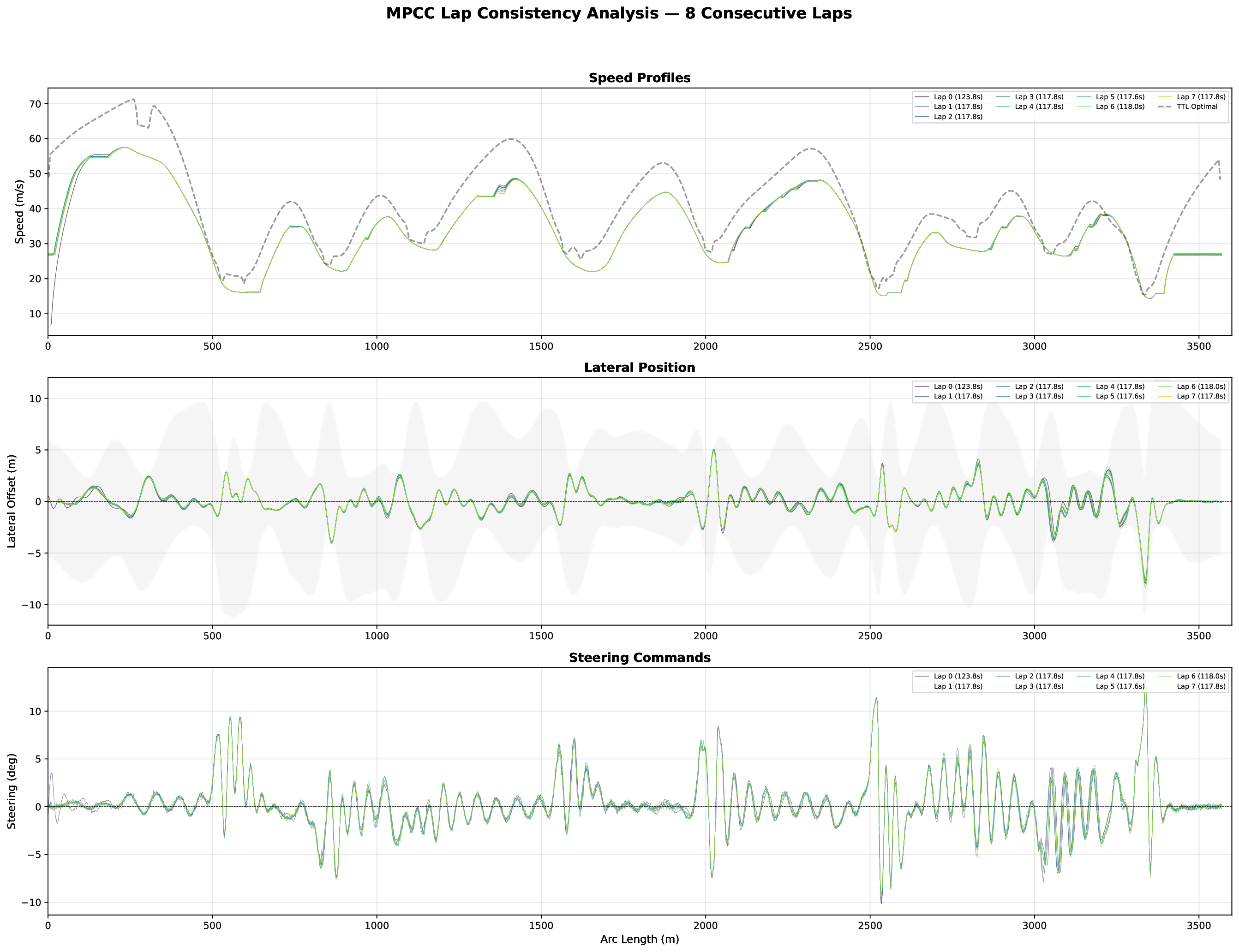
Lap consistency (left): across 8 consecutive laps, speed profiles, lateral position, and steering commands are tightly overlapping, confirming that closed-loop MPC produces repeatable behavior without drift.
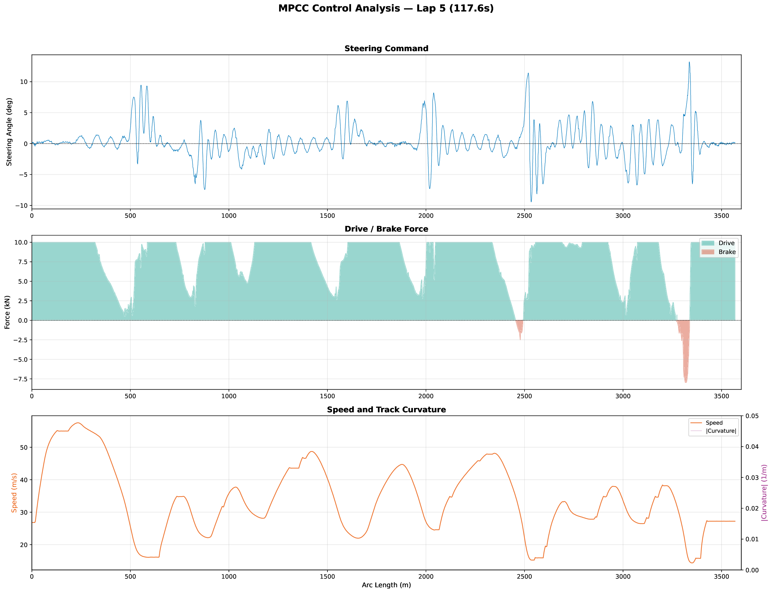
Control analysis (best lap, 117.6 s): The drive/brake panel shows the trail-braking pattern the combined-slip tire model enables: sharp braking zones at corner entries, maximum drive on straights. Speed (orange) is tightly anti-correlated with curvature (pink), confirming the progress-maximizing objective is working as intended.
Track Testing
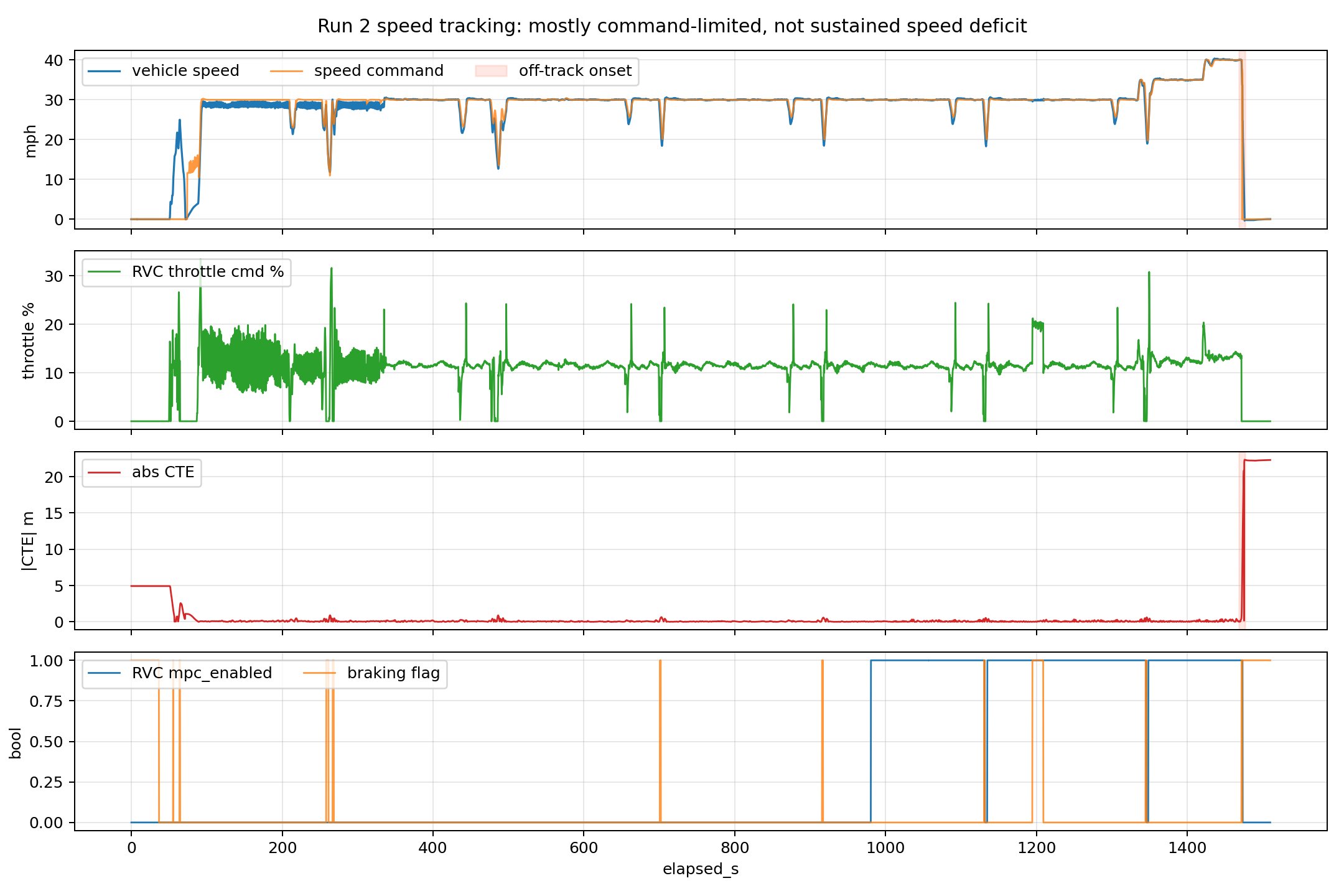
We ran the controller on the physical Dallara AV-24 at a closed track. Run 2 shows the vehicle tracking a 40 mph speed command with low cross-track error across multiple laps (~1,400 seconds). The off-track event visible at the end was caused by a throttle command conflict; the torque safety filter (preventing simultaneous front braking and rear acceleration) was not yet handling the edge case where resolver cores were reduced from 6 to 1 (done to reduce solve-time variance). The cross-track error remained under 2 m for the entire run until the final upset, which speaks to the robustness of the tracking.
Takeaways
The project demonstrates that progress-maximizing NMPC is viable for real autonomous racing. Key lessons:
- Timescale separation works. Solving the lap-planning problem once offline with a high-fidelity double-track model, then querying the result as a TTL during online control, gives each layer exactly the model fidelity it needs without compromising the other’s timing requirements.
- Solver conditioning is everything. Variable scaling, eigenvalue regularization, and aggressive warm-starting are not optional polish; they are what makes a single Newton step reliable in a nonconvex problem.
- The 50× warm-start bug illustrates how non-obvious numerical issues can hide behind seemingly correct implementations. Exact derivatives from CasADi were essential for diagnosing it.
- TDD at 3.3× test density allowed the architecture to evolve through several major iterations without regressions, essential in a safety-critical codebase where a wrong actuator command means an off-track event at 200 km/h.
Related projects
MPC for UR7e Robotic Arm: Warehouse Sorting
Constrained joint-space Model Predictive Control for a UR7e manipulator. An RGB-D perception pipeline localizes objects and obstacles; a receding-horizon CasADi/IPOPT solver generates collision-free joint trajectories at 12 Hz, validated in MuJoCo and deployed on real hardware.
Decentralized Fleet Coordination for Airport Ground Operations
Multi-agent coverage control for airport ground vehicles using Buffered Voronoi Cells, Lloyd's algorithm, and game-theoretic demand response. Zero collisions across all test scenarios.
Multi-Agent RL for Autonomous Driving in Waymax
PPO agent trained in Google's JAX-based Waymax simulator on Waymo Open Dataset traffic. Began as speed tracking on log-replay traffic and ended as adaptive cruise control evaluated on a five-scenario stress suite: stalled vehicle, slow lead, emergency braking, stop-and-go, and cut-in. Four pass with zero contact; the fifth exposes a measurable generalization gap. Fourteen training runs, ten documented failure modes.