MPC for UR7e Robotic Arm: Warehouse Sorting
Constrained joint-space Model Predictive Control for a UR7e manipulator. An RGB-D perception pipeline localizes objects and obstacles; a receding-horizon CasADi/IPOPT solver generates collision-free joint trajectories at 12 Hz, validated in MuJoCo and deployed on real hardware.
Demo
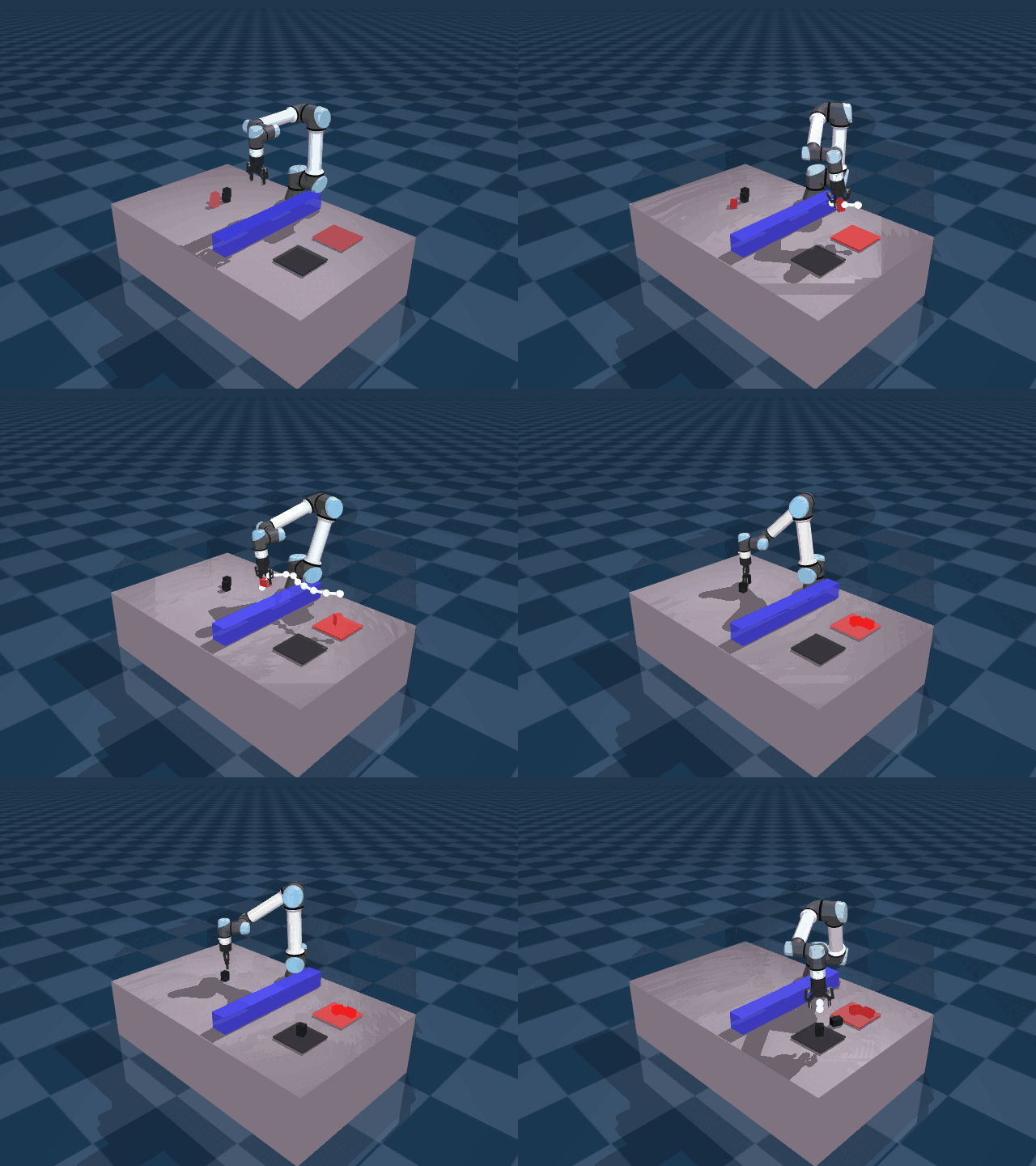
The same MPC pipeline running in simulation and on the physical UR7e. The receding-horizon solver replans every control tick: no hand-coded waypoints, no pre-scripted trajectories. The arm detects cube colors via an RGB-D camera, plans a collision-free joint-space path around the obstacle bin, grasps each cube, and drops it in the correct zone.
System Architecture
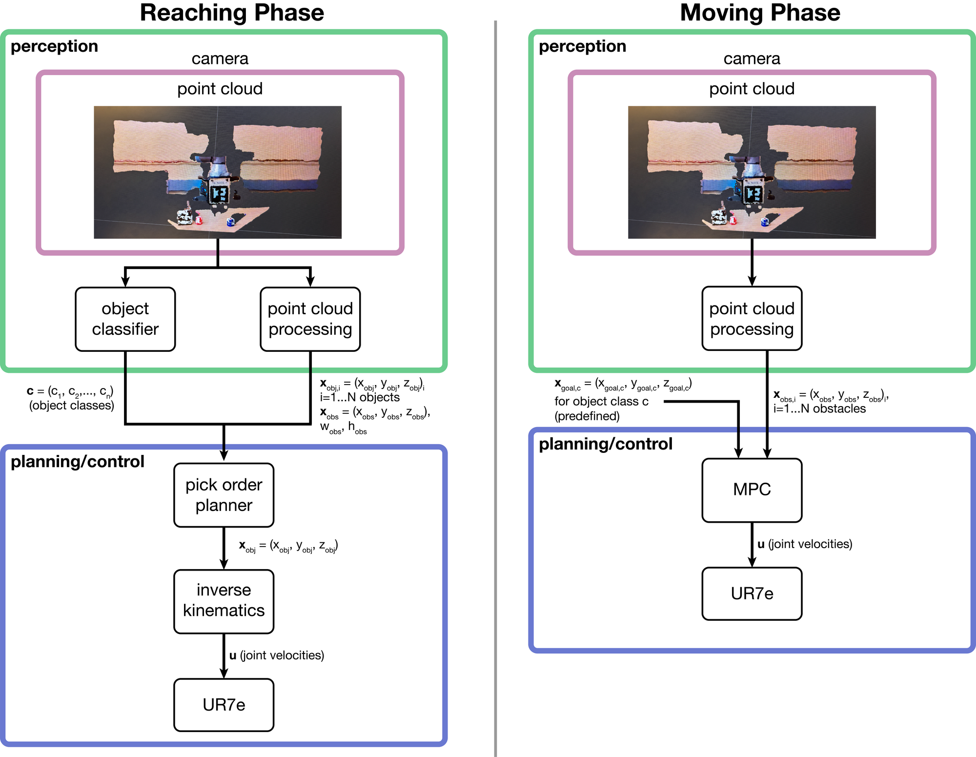
The system operates in two alternating phases that share the same perception stack but use different controllers.
Reaching Phase: the arm moves to a grasp pose. The RGB-D point cloud feeds into an object classifier (identifying cube colors ) and a point cloud processor (localizing object positions and the obstacle bounding box ). A pick-order planner selects the next target cube and passes its 3D position to an inverse kinematics solver, which computes a target joint configuration . Joint velocities drive the UR7e to that pose.
Moving Phase: MPC takes over for the transport. The camera continuously updates the obstacle AABB and the predefined goal positions for each color class. The MPC solves a receding-horizon optimization each tick and outputs joint velocity commands to carry the held cube to the drop zone while maintaining obstacle clearance throughout the trajectory.
Physical Setup
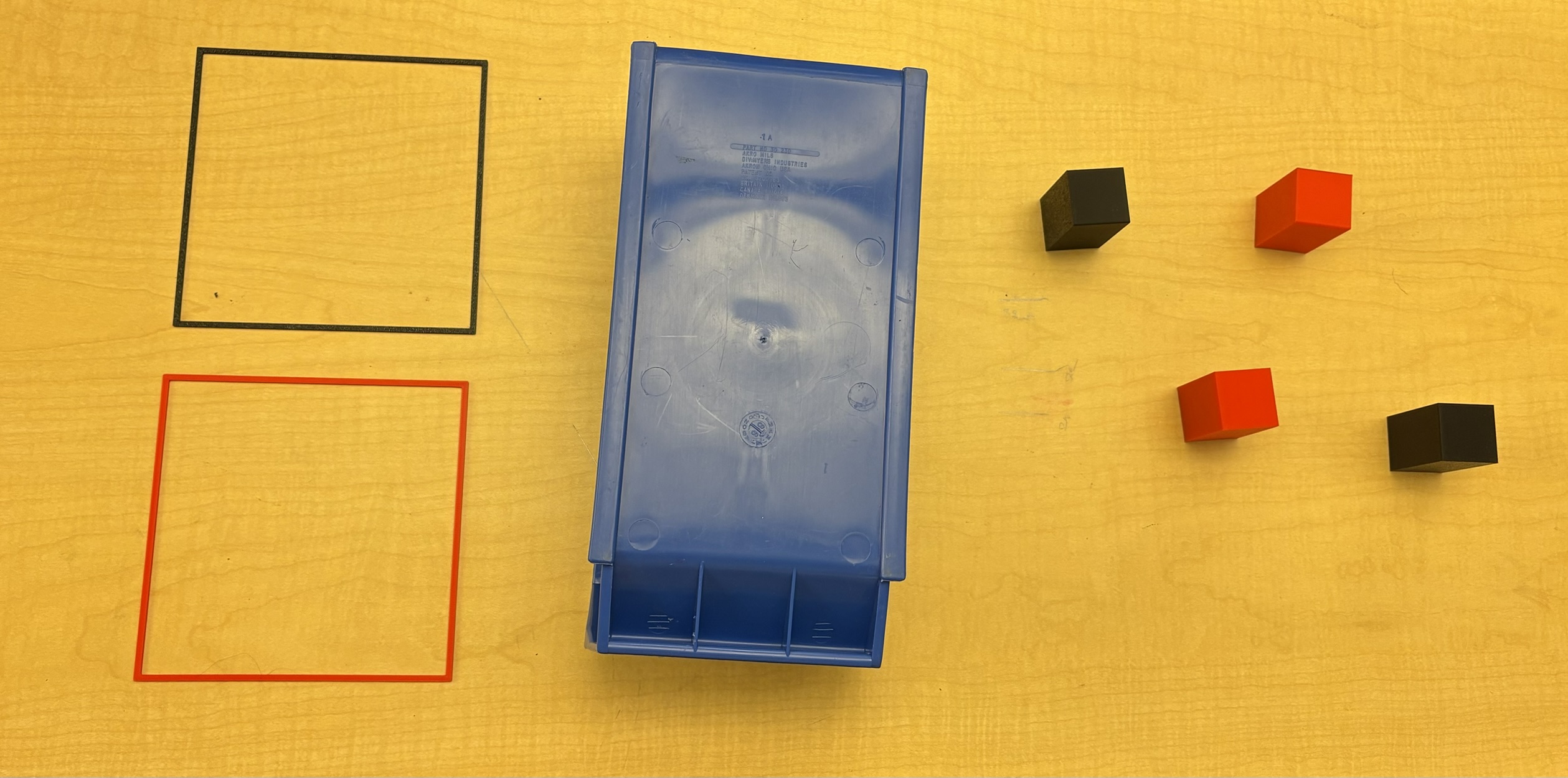
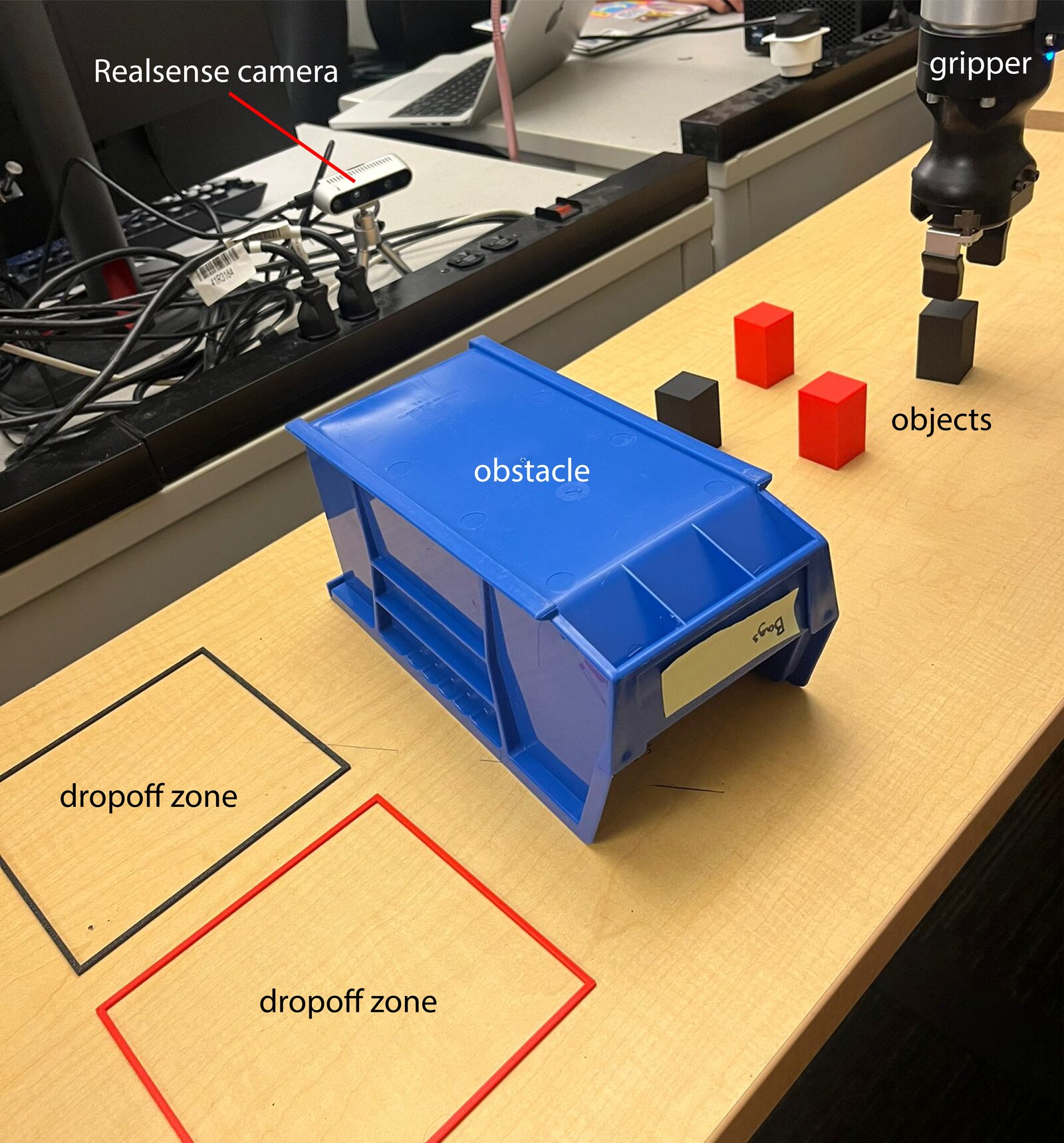
The workspace has multiple red and black cubes, a rigid blue plastic bin acting as the obstacle, and two rectangular drop zones marked on the table surface. An Intel RealSense RGB-D435i camera is mounted overhead to stream point-cloud and color data. The UR7e carries a Robotiq 2F-85 parallel-jaw gripper. The obstacle is deliberately positioned between the pick region and the drop zones, so the arm must always plan a non-trivial detour, which makes straight-line Cartesian planning insufficient and validates the MPC’s obstacle avoidance behavior.
Perception: RViz Visualization
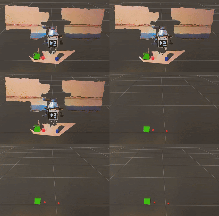
The perception node processes the RealSense depth stream in real time. DBSCAN clustering segments the point cloud into individual objects, and axis-aligned bounding boxes (AABBs) are fit to the obstacle cluster. Color classification assigns each cube to a class. The RViz visualization shows published cube positions and the inflated obstacle AABB before y-axis extension; the colored markers correspond to detected red and black cubes, and the transparent box is the inflated obstacle region passed directly into the MPC collision constraint.
MPC Formulation
The MPC operates in joint space. The state at discrete time is the 6-DoF joint configuration , and the control input is a bounded joint position increment . The prediction model is a simple integrator:
with sample period and prediction horizon steps. Choosing joint position increments (rather than joint velocities or Cartesian targets) keeps the prediction model linear and lets joint limits be enforced as hard box constraints directly on the optimization variables.
Cost Function
At each control cycle the MPC minimizes:
where is the end-effector position from forward kinematics, is the desired drop position (computed via IK), , , and (a heavier terminal weight to drive convergence to goal). The slack terms and soften the orientation and table-clearance constraints to maintain solver feasibility under perception noise.
Constraints
(i) Joint limits and step bounds:
The per-step bound of directly reflects the position-increment interface of the UR7e’s low-level controller, approximating actuator velocity limits.
(ii) Obstacle avoidance. The gripper and grasped object are approximated by three proxy spheres centered at , , in the tool frame, each with inflated radius . At every horizon step the Euclidean distance from each sphere center (computed via forward kinematics) to the obstacle AABB must satisfy:
The instantaneous obstacle clearance margin is . Collision-free motion corresponds to .
(iii) Table clearance. A soft vertical floor constraint prevents the arm from colliding with the tabletop during transport, relaxed via slack :
The effective floor height is phase-dependent: stricter on descent to the grasp pose, relaxed during transport to allow the arm to skim over the obstacle.
(iv) Terminal orientation. A down-facing tool-frame orientation is enforced softly only at the terminal step via slack . Intermediate orientation is left unconstrained, which gives the optimizer freedom to find non-obvious collision-avoiding paths without locking the gripper angle along the entire trajectory.
Receding Horizon Implementation
Rather than applying only the first computed increment (standard MPC), the first three increments ( of motion) are executed before replanning. This reduces solver invocation frequency while keeping responsiveness adequate for the task. The loop terminates when or after 40 solver iterations. Warm-starting with the previous horizon solution is the primary driver of the ~3× speedup from cold to steady-state solve time.
MuJoCo Simulation
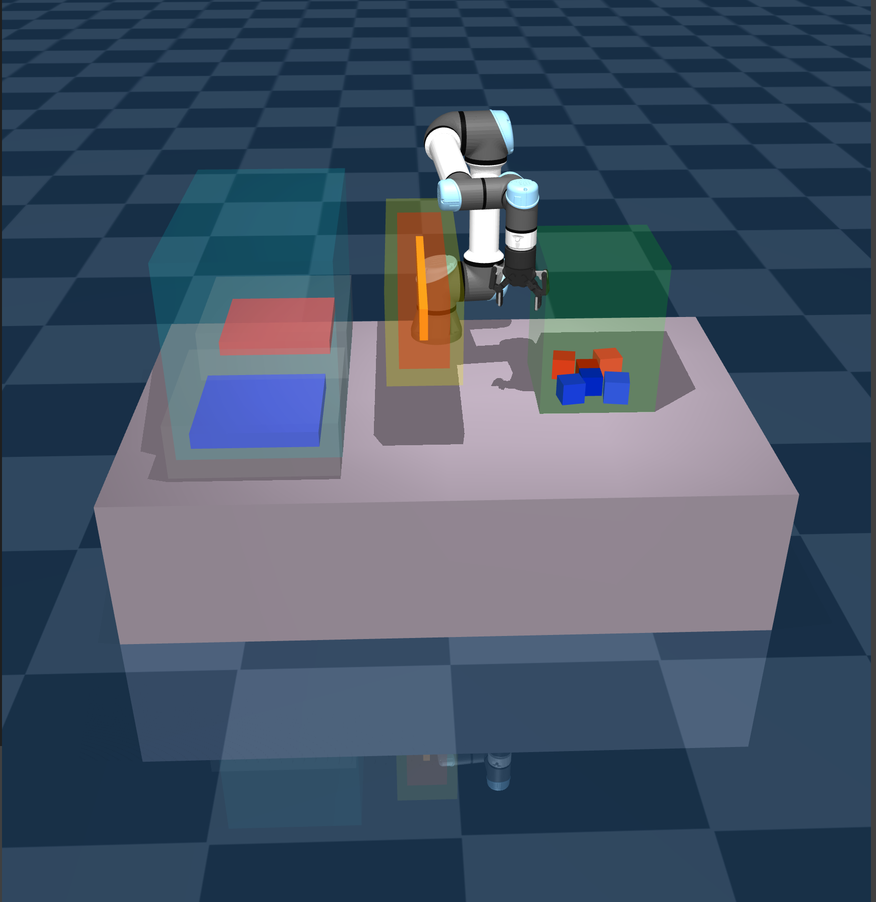
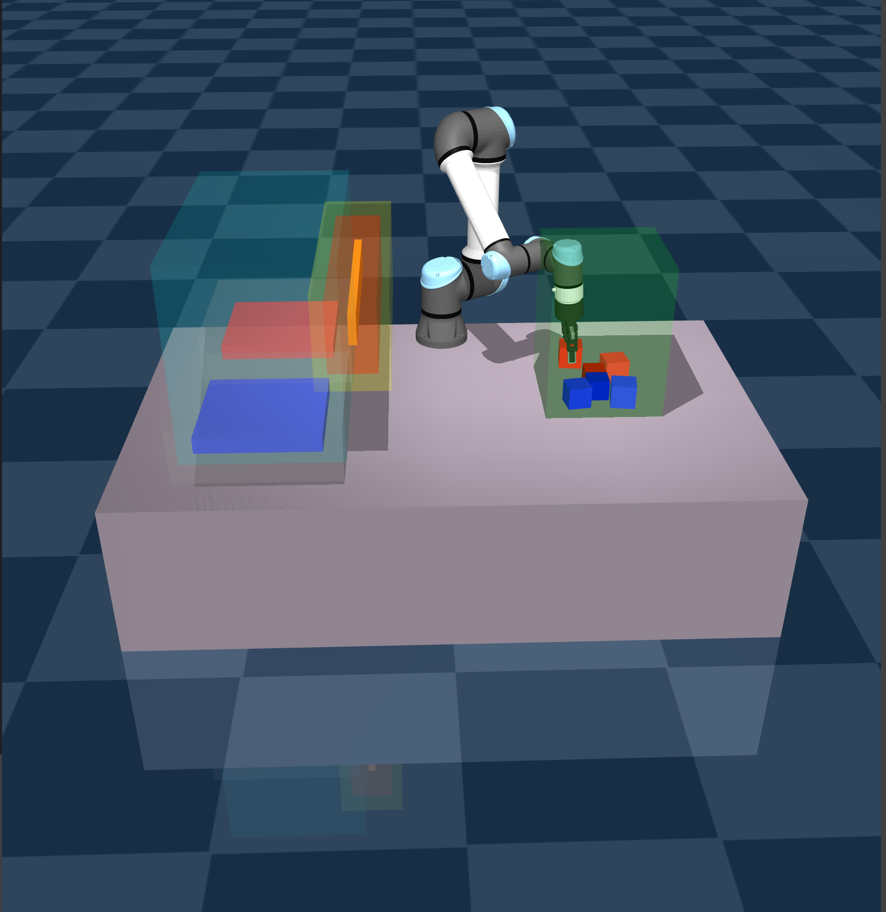
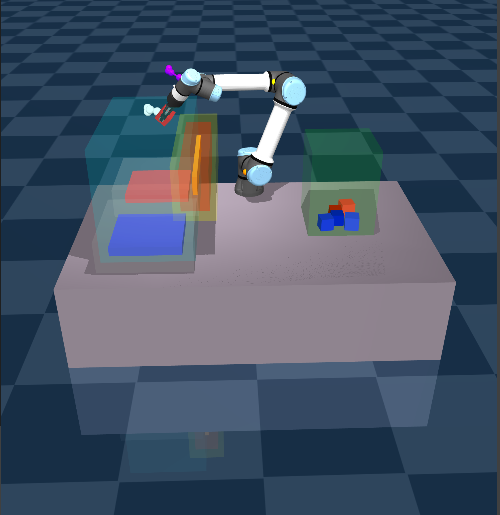
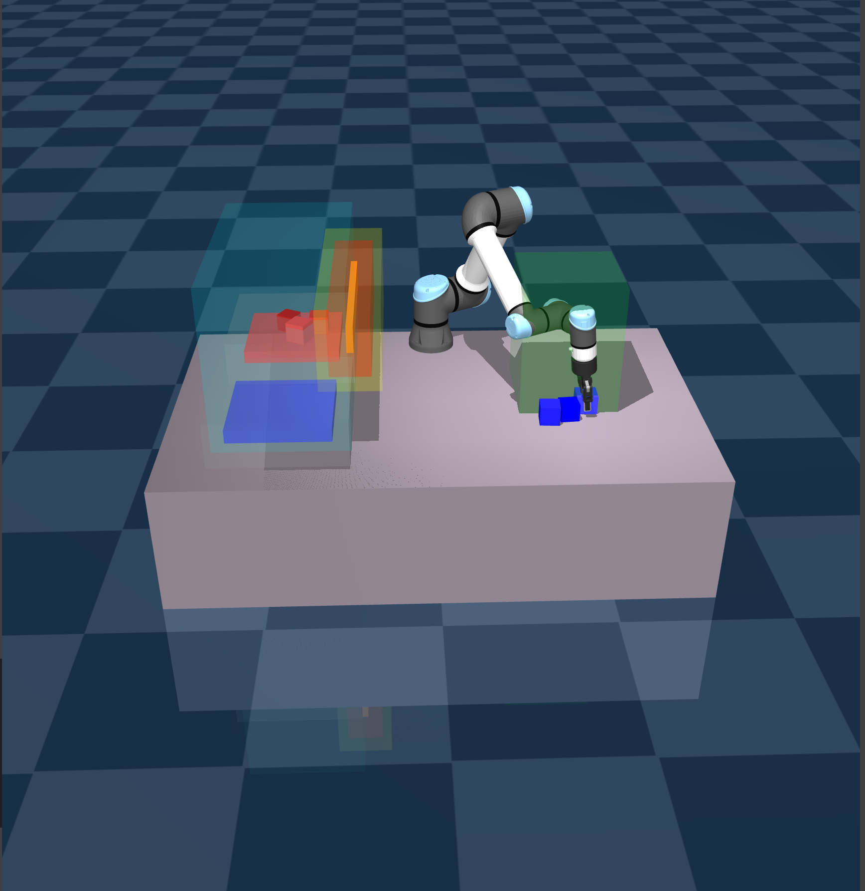
The MuJoCo environment mirrors the real lab setup: colored drop zones, the static obstacle bin, and a Robotiq gripper. The cyan markers visualize the MPC’s predicted end-effector path over the horizon steps in real time. The four frames show the full task sequence: approach, grasp, obstacle transit, and placement.
Results on Real Hardware
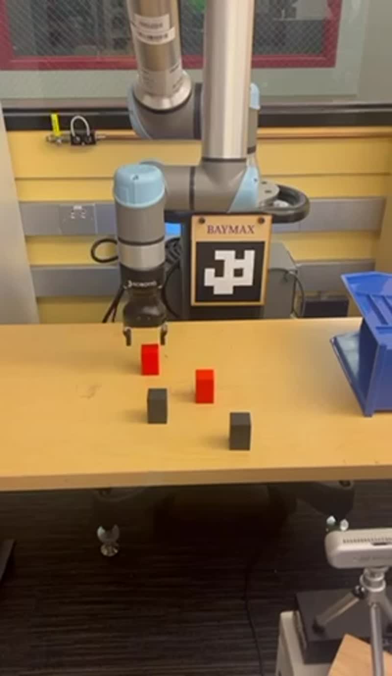
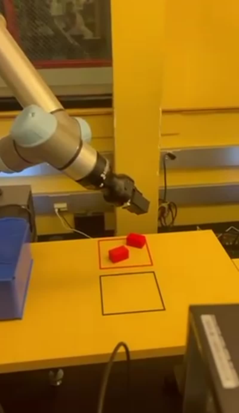
Red cubes in the red zone, black cubes in the black zone: fully autonomous end-to-end. The arm reclassifies each cube’s color from the live camera feed, routes around the obstacle bin, and places each cube in the correct zone with no human intervention between picks.
Trajectory Analysis
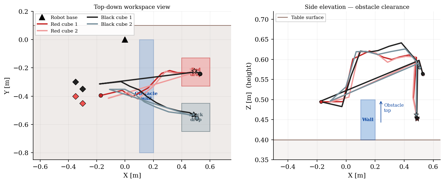
The executed end-effector Cartesian trajectory (blue) for a representative transport phase. Starting from the initial grasp pose (green dot), the MPC generates a smooth path that intentionally arcs around the obstacle AABB (red box) before converging to the target drop position (red ×). The detour is not hand-coded; it emerges from the obstacle clearance constraint at each horizon step. At no point does the optimizer force a fixed height; the arm finds its own clearance strategy, trading off goal progress against constraint satisfaction at every tick.
Convergence & Safety
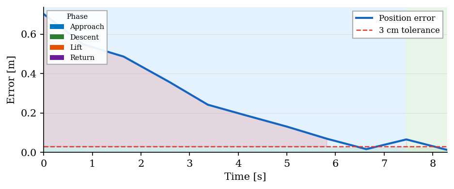
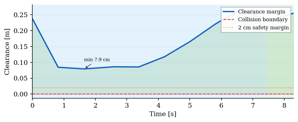
The end-effector position error decreases steadily from an initial offset of to within the stopping tolerance. Small non-monotonic fluctuations near convergence are expected in closed-loop MPC; each replan trades off goal progress against the obstacle and table constraints, so the path is not strictly greedy. The obstacle clearance margin remains strictly positive throughout the entire trajectory, confirming collision-free behavior even during the obstacle detour. The soft slack variables prevent constraint infeasibility under perception noise without relaxing the hard obstacle constraint.
Joint Profiles & Solve Time
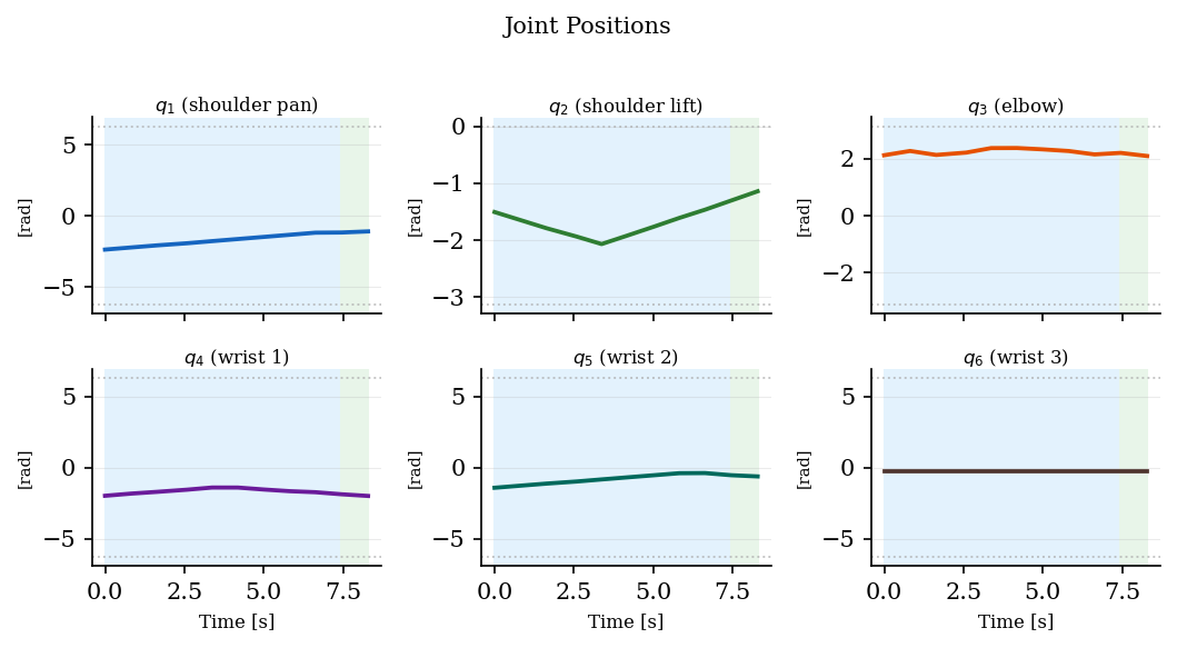
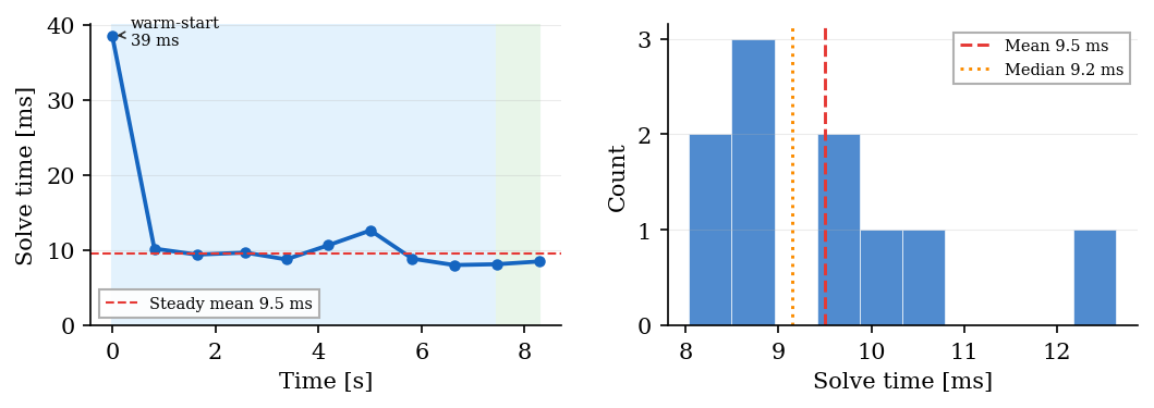
Joint increment commands remain within the enforced per-step bounds across all six joints throughout the trajectory, with no aggressive joint motion, consistent with the position-increment interface assumption. Solve time drops from on the cold start (no prior solution to warm-start from) to a steady-state mean of , well within the control timestep (). Warm-starting with the previous horizon’s solution is the dominant factor in the speedup; the optimizer starts already near the previous optimum and converges in far fewer IPOPT iterations.
Related projects
Nonlinear MPC for Autonomous Racing
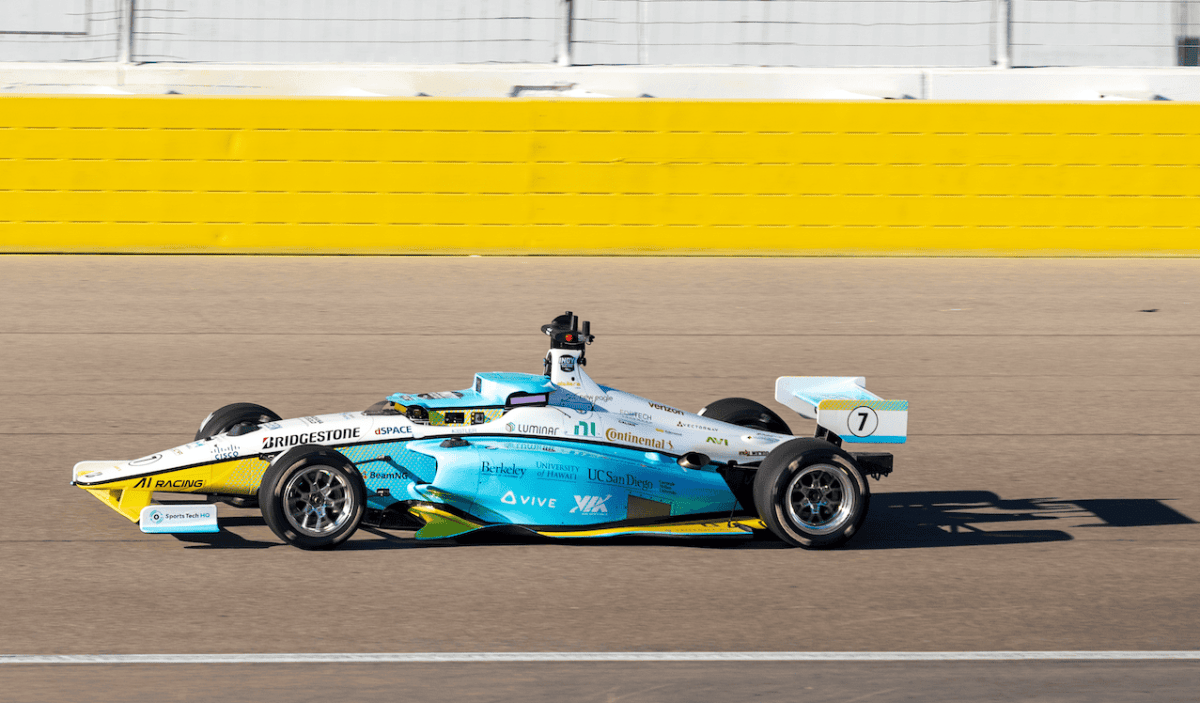
Progress-maximizing NMPC for a full-scale Dallara AV-24 competing in the Indy Autonomous Challenge. Two-timescale architecture: a full-lap minimum-time NLP solved offline with a double-track Pacejka vehicle model produces the Track Trajectory Library, while an NMPC at 100 Hz in a Frenet frame executes it with RTI. Validated in AWSIM (best lap 117.6 s, 207 km/h max) and on the physical car.
Decentralized Fleet Coordination for Airport Ground Operations
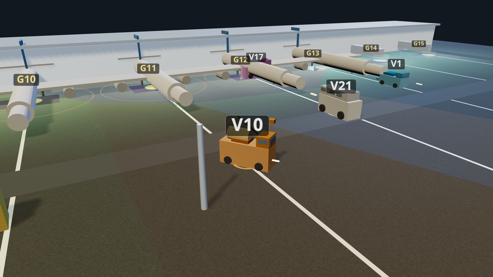
Multi-agent coverage control for airport ground vehicles using Buffered Voronoi Cells, Lloyd's algorithm, and game-theoretic demand response. Zero collisions across all test scenarios.
 research
 Does a Merge Planner Need a Model of the Traffic?
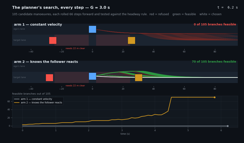
Three planners share one control interface and differ only in what they believe about the car behind them: nothing, everything, or whatever they can learn. Across 41,130 episodes on 914 held-out Waymo scenes, a correct model of the follower is worth everything in one narrow band of gap sizes and nothing outside it, and the moment it is wrong, the planner that trusted it drops to zero. A learned policy wins the opposite regime, but a control proves it wins by acting early rather than by understanding anything.