Decentralized Fleet Coordination for Airport Ground Operations
Multi-agent coverage control for airport ground vehicles using Buffered Voronoi Cells, Lloyd's algorithm, and game-theoretic demand response. Zero collisions across all test scenarios.
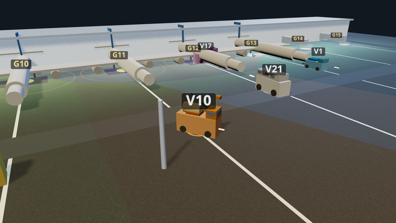
Airport aprons run on tight tolerances. A delayed fuel truck cascades into a gate conflict; a misrouted baggage tug holds an aircraft at the jetbridge. At scale, centralized dispatch becomes the bottleneck; every new gate or vehicle makes the assignment problem harder. This project designs a fully decentralized coordination stack for airport ground-support vehicles: each agent sees only its local neighbors, computes its own service target, and filters its own motion for safety. The fleet self-organizes. No dispatcher required.
The final 16-vehicle, 32-gate simulation satisfies every safety constraint (zero vehicle-to-vehicle collisions, zero obstacle penetrations) while converging to within 8% of the centralized coverage optimum.
The Apron
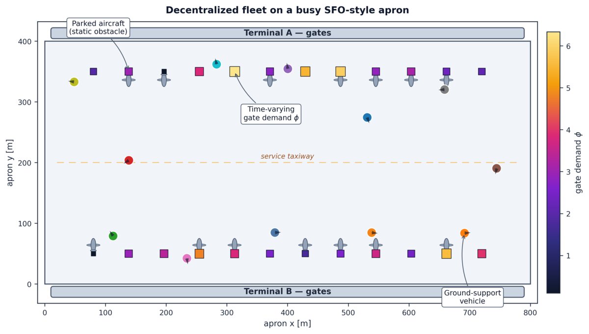
The environment is an SFO International Terminal apron modeled as a rectangular domain with gates split across two terminal rows and a service taxiway running between them. The fleet has heterogeneous ground vehicles (fuel trucks, baggage tugs, catering lifts, and GPU units), each with planar position .
The first design decision is where to send vehicles. Gates and parked aircraft are static obstacles, not drivable targets, so each gate is mapped to an apron-side service standoff point:
Vehicles converge toward these approach positions, close enough to serve the gate and far enough to avoid the aircraft footprint. The combined coverage domain adds a background density grid so vehicles spread across open apron space between demand events.
System Architecture
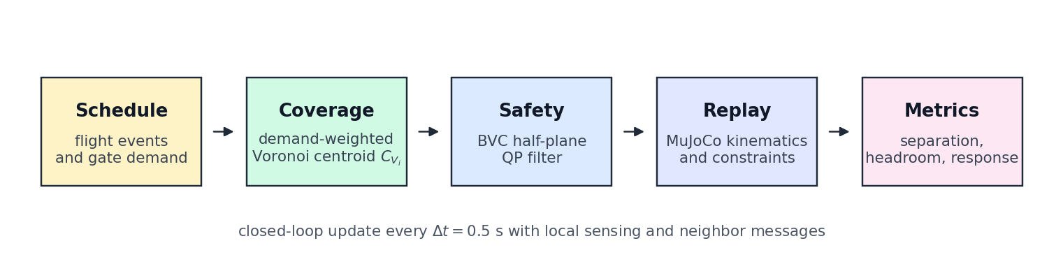
The control loop runs at using only local sensing and neighbor messages. Each tick: flight events update gate demands; each vehicle computes its Voronoi cell and demand-weighted centroid; the BVC quadratic program projects that centroid command to a collision-free velocity; and the command is integrated through the MuJoCo physics layer. Separation, clearance, and kinematic diagnostics are logged throughout.
The architecture has no shared state, no global solver, and no communication beyond pairwise position sharing with local neighbors within .
Coverage Control
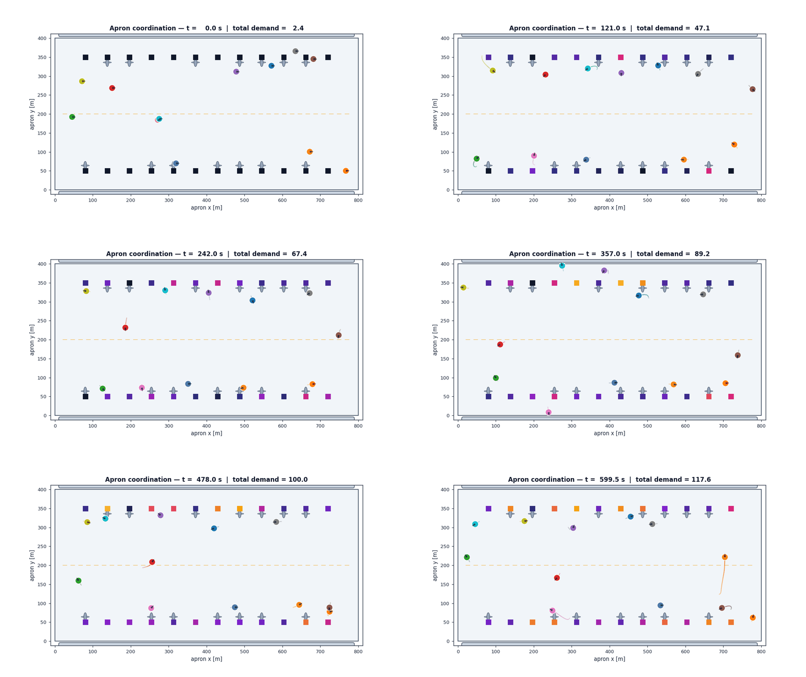
Gate demand changes continuously: a flight lands and eight service vehicles are needed at once; thirty minutes later that gate is quiet and three others are busy. The coverage controller tracks this without any explicit task assignment.
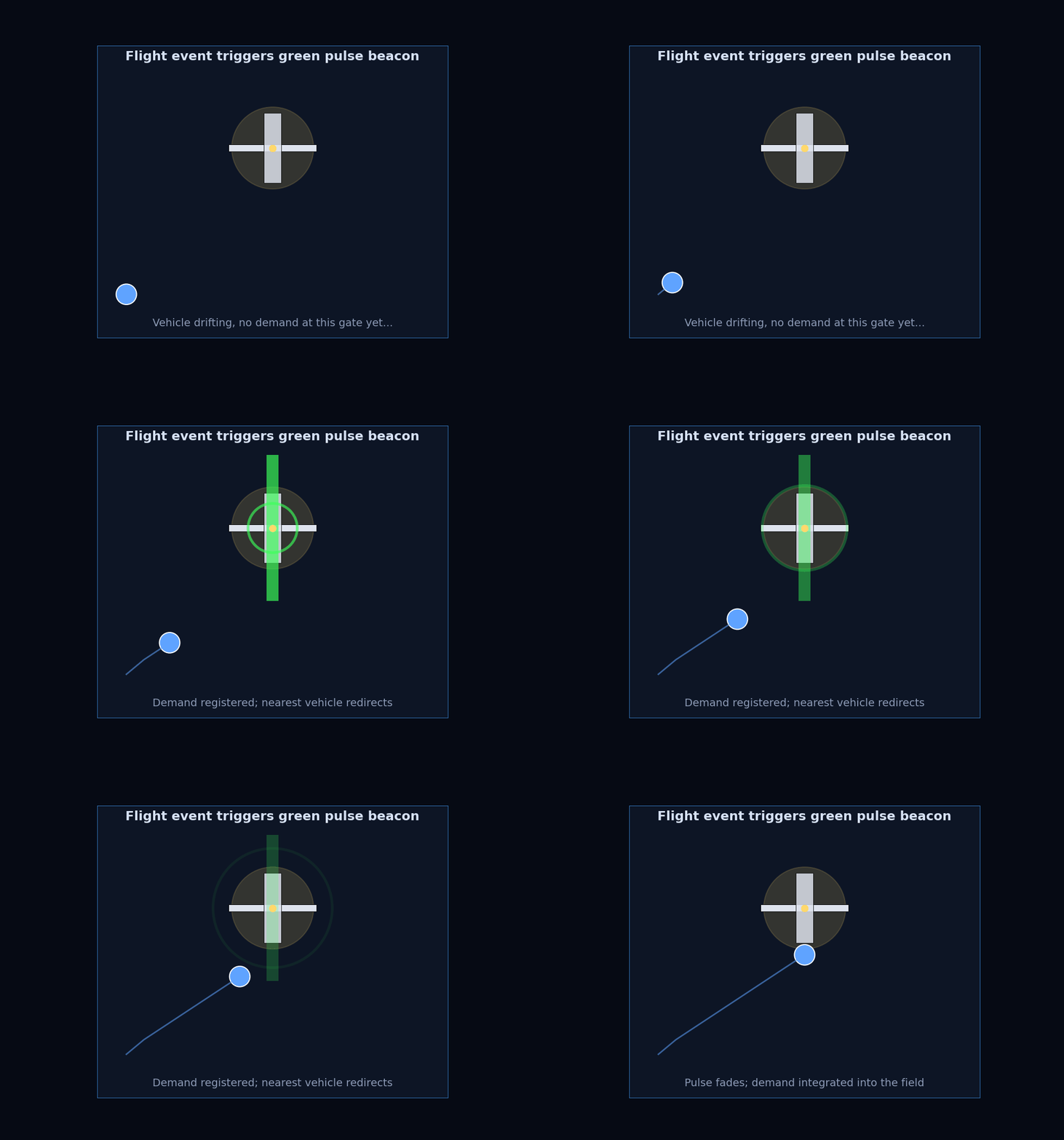
Each gate carries a service demand that spikes on flight arrival and decays exponentially:
The coverage objective is the demand-weighted quantization cost, a measure of how far high-demand gates are from the nearest vehicle:
where is vehicle ‘s Voronoi cell and is the demand density at point . Minimizing drives vehicles toward high-demand regions.
Lloyd’s algorithm gives the gradient descent step: move each vehicle toward the demand-weighted centroid of its Voronoi cell,
The command is speed-capped and tapered as the vehicle approaches its centroid to prevent overshoot near convergence:
This is the desired command before safety filtering.
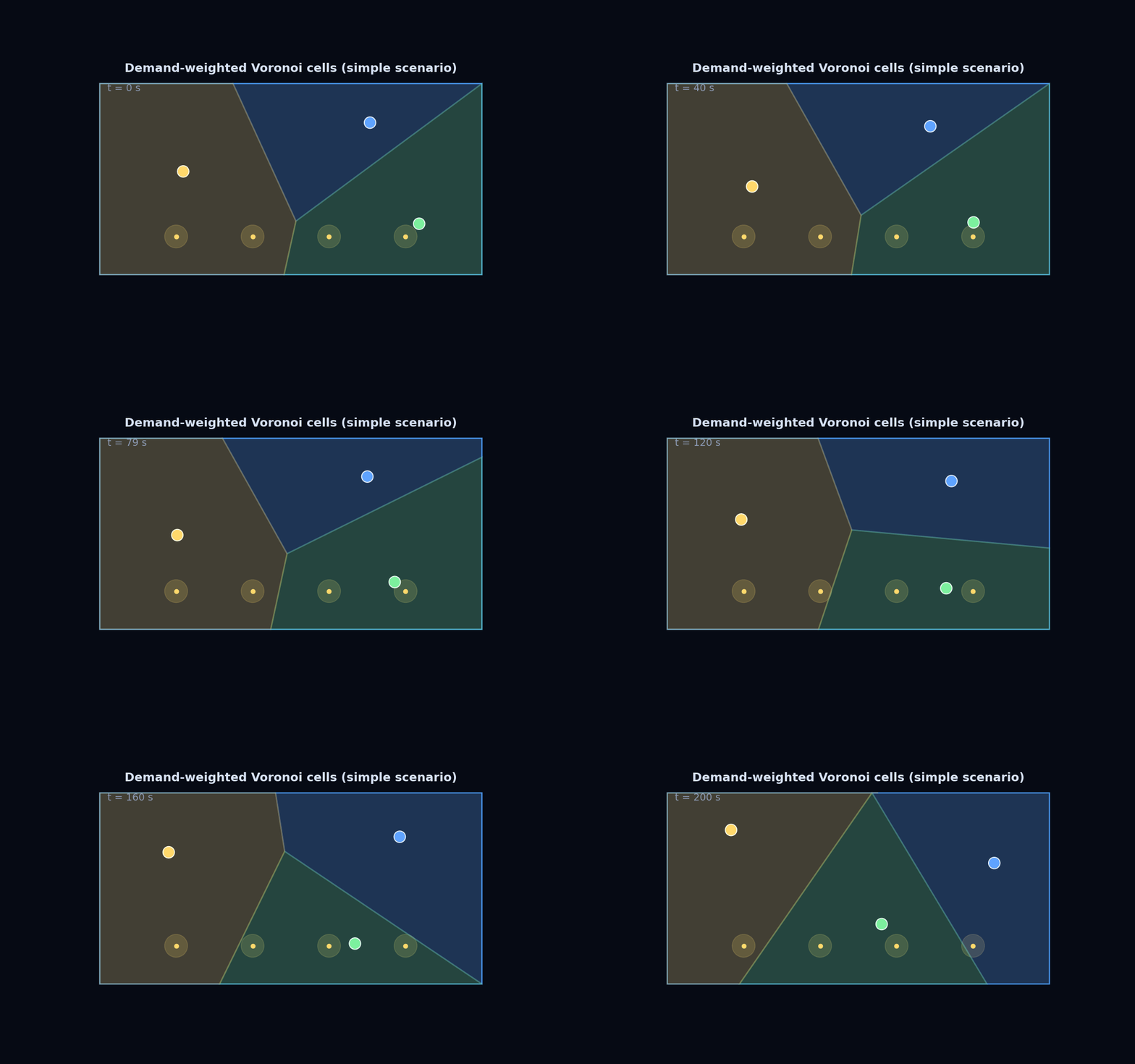
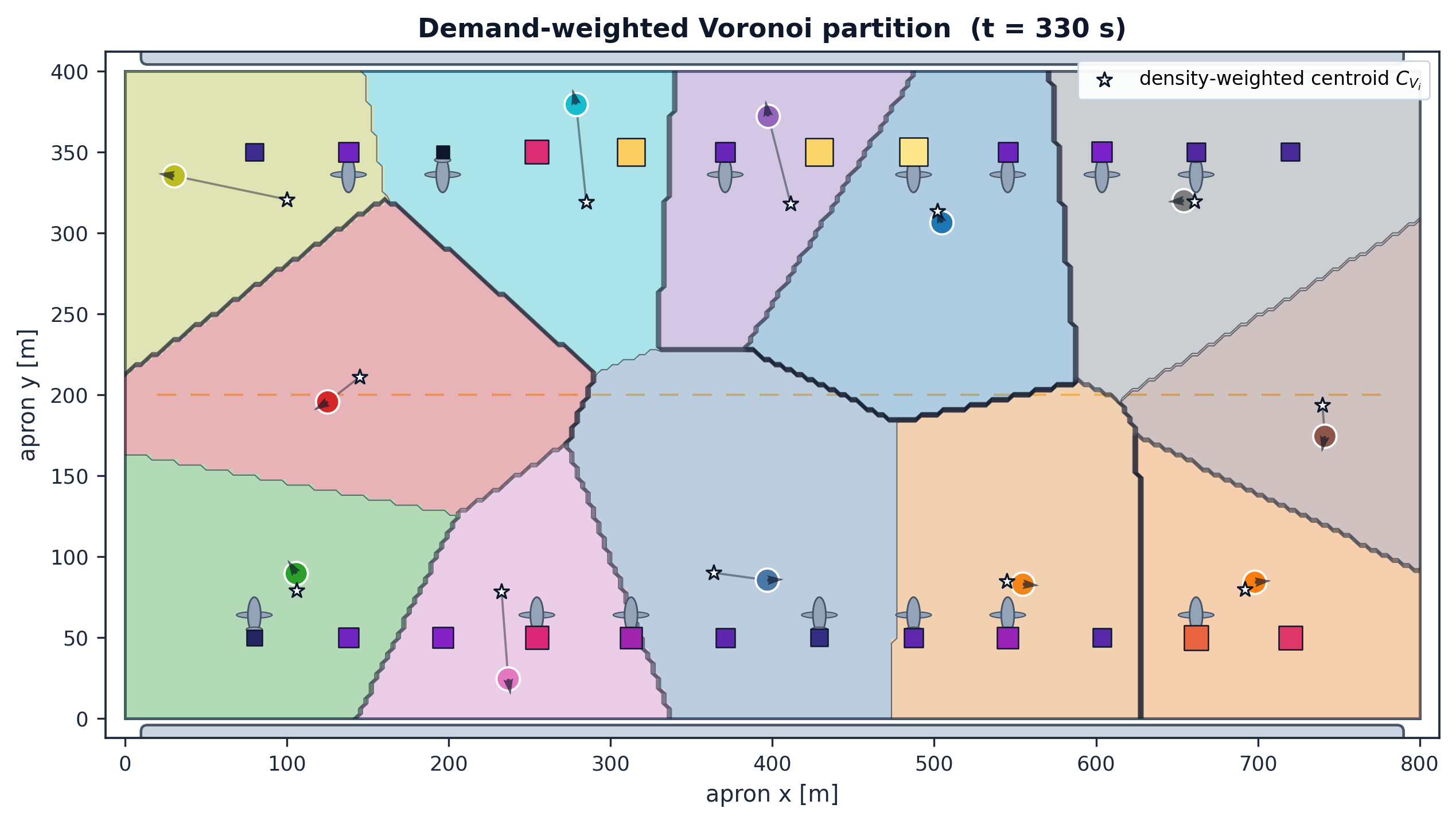
The snapshot at shows cell boundaries biased toward high-demand gates; the density-weighted centroid (star markers) sits closer to busy gates than to the geometric cell center. Vehicles chase their moving centroid targets; cells reform on every tick. No agent ever needs to know the global demand state.
Collision Avoidance
The coverage law alone says nothing about collisions. Rather than stacking a separate avoidance layer on top, the design uses Buffered Voronoi Cells, a safety filter that wraps the coverage command in a convex QP. The result is a single optimization per vehicle per tick that simultaneously targets the coverage objective and guarantees collision freedom.
For vehicle with neighbor , the BVC halfplane constrains the next position :
where is the safety radius. Any velocity whose resulting lies inside the Buffered Voronoi Cell is provably collision-free. The safety-filtered command is the smallest deviation from that satisfies all neighbor halfplanes:
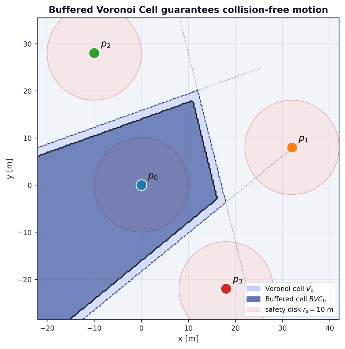
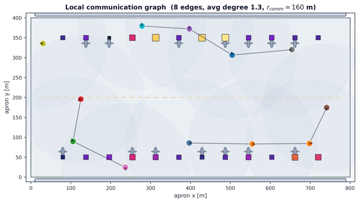
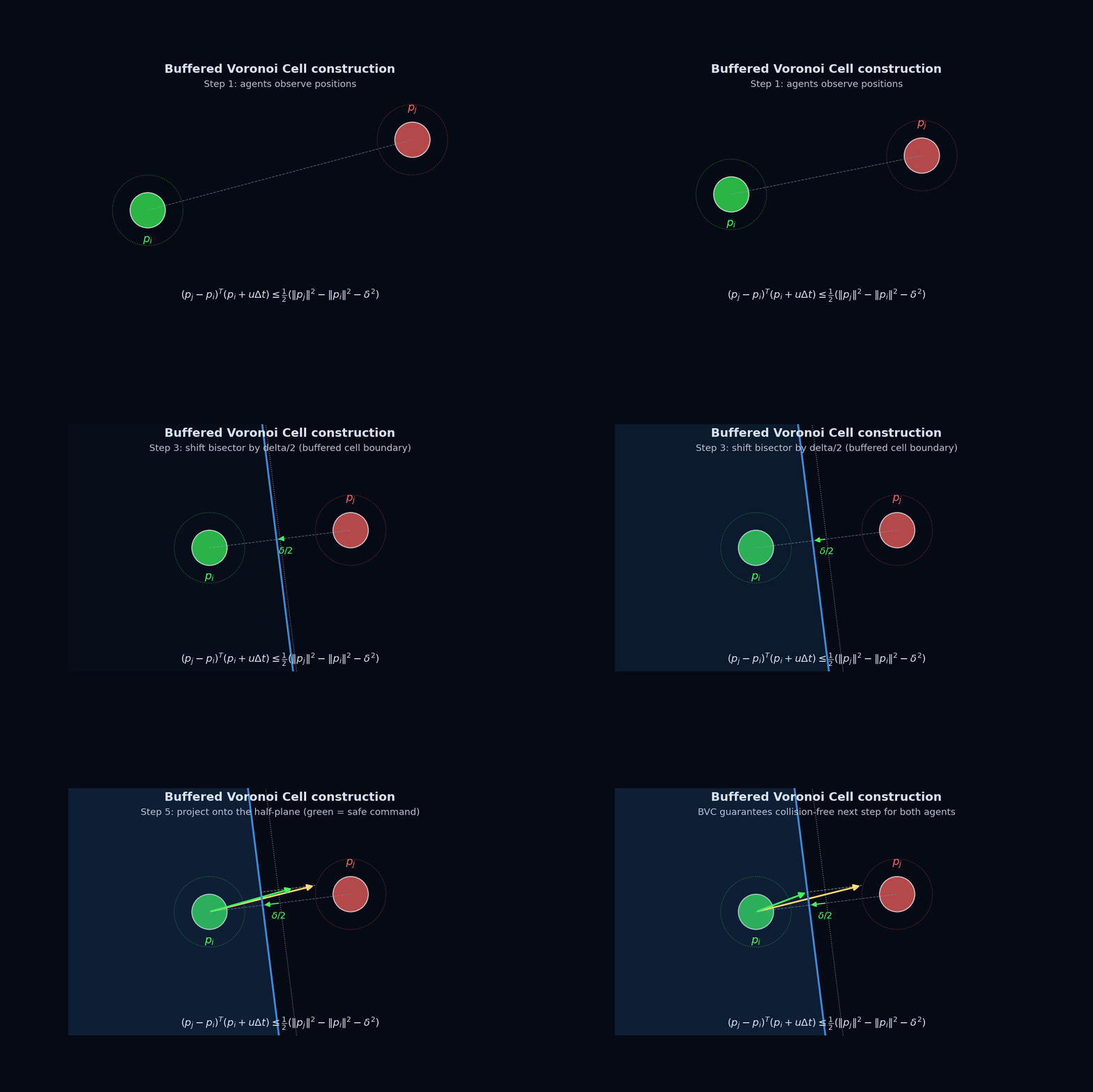
The BVC construction (left) shows three neighbor halfplanes carving the safe feasible region out of the full Voronoi cell ; any command landing in the dark region is provably safe. The communication graph (right) shows why the approach scales: each vehicle only shares positions with local neighbors within 160 m, averaging 1.3 neighbors per agent. There is no broadcast, no global state.
Gates and parked aircraft add a second class of static exclusion zones with radii for gates and for parked aircraft. Each nearby obstacle contributes a tangent halfplane to the QP: , where .
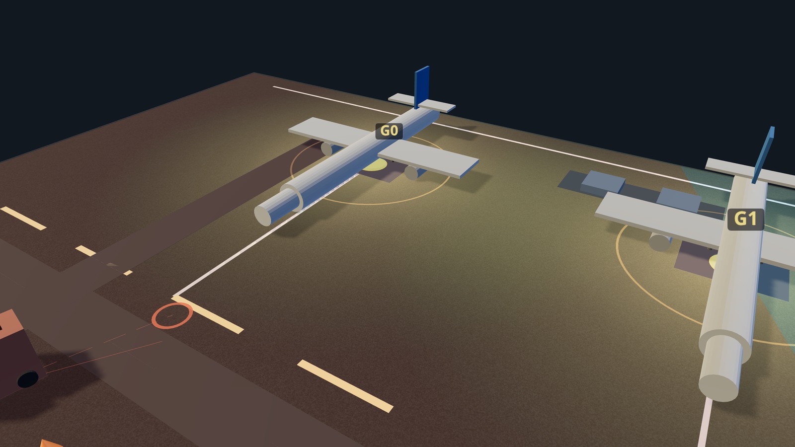
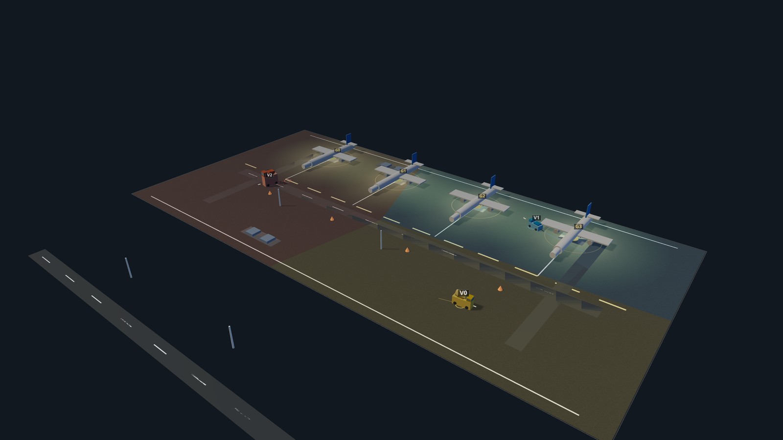
The gate-level view shows the exclusion zones in practice: vehicles approach gates from the apron side, held back from the aircraft footprint by the obstacle halfplane constraints. The demand-field glow at each gate shows where centroid targets are pulling them.
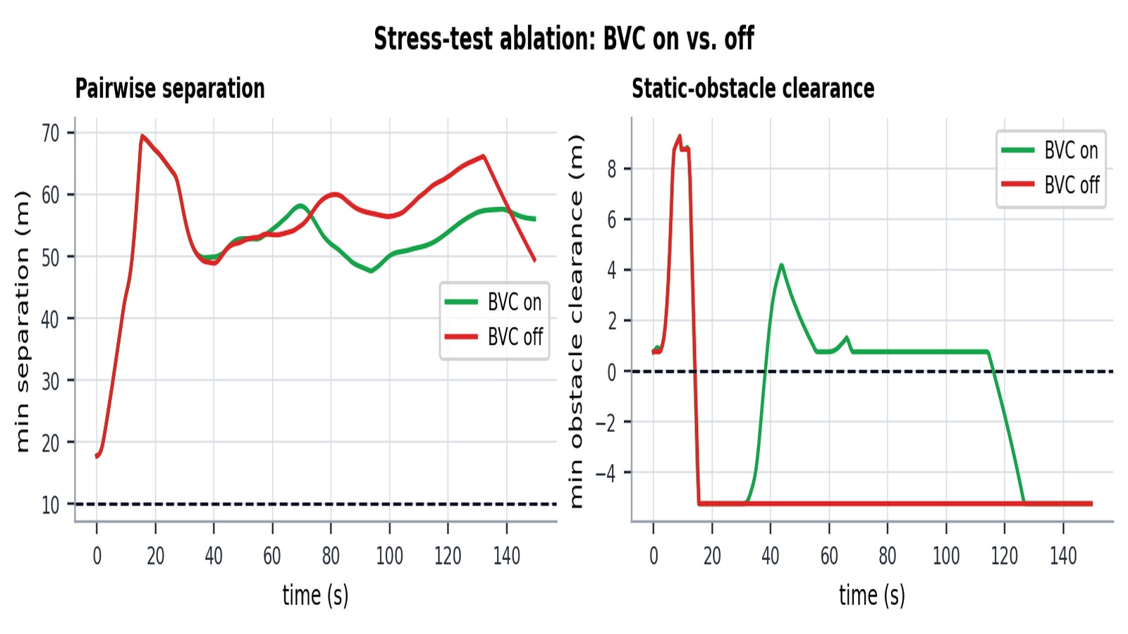
The ablation runs the same stress scenario with and without BVC. Without it, vehicles penetrate static obstacles within the first 20 seconds: clearance drops to −4 m and never recovers (red). With BVC on, pairwise separation stays above the 10 m safety limit and obstacle clearance remains strictly positive throughout (green). The safety guarantee holds in practice, not just in theory.
Simulation
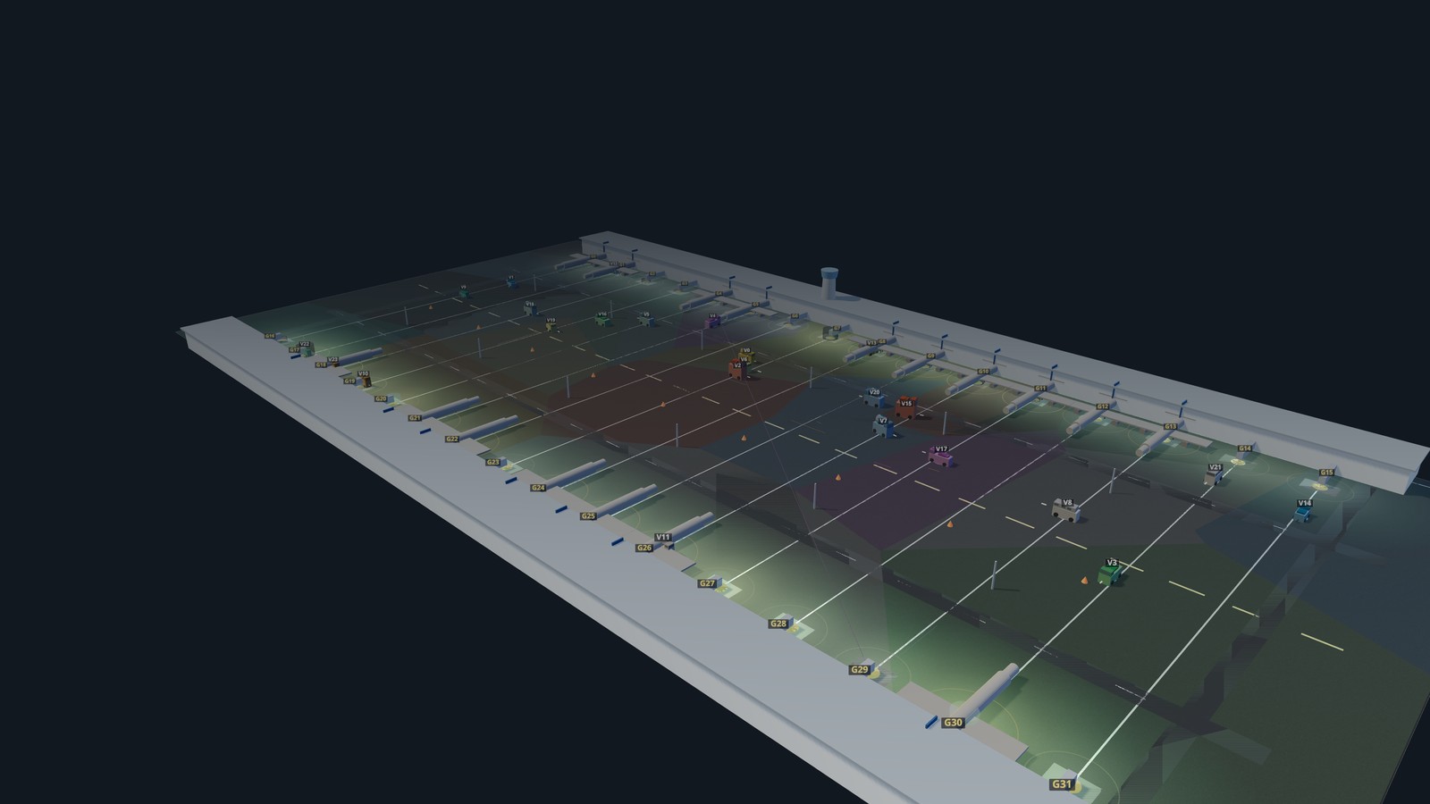
The full simulation runs 16 vehicles on the 32-gate SFO layout with MuJoCo integrating the force/torque dynamics. Each vehicle state is ; a first-order smoother low-passes the BVC output before it enters the physics layer, and longitudinal and lateral force controllers track the smoothed command while a yaw torque controller drives heading:
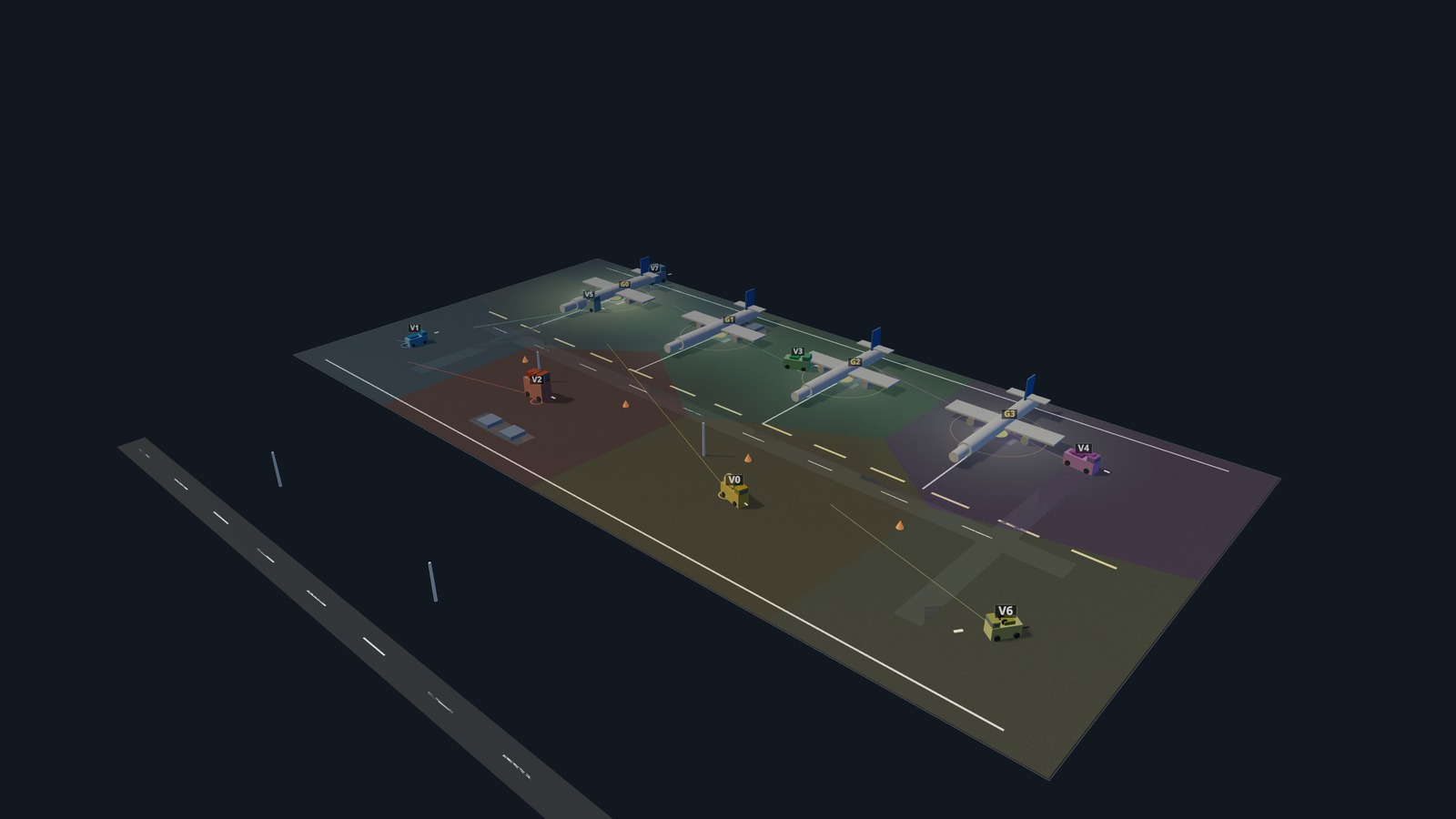
The 3D replay visualizes the same MuJoCo trajectory in a browser viewer: Voronoi cell boundaries, BVC circles, demand overlays, and vehicle labels are all rendered live from the logged state sequence.
Results
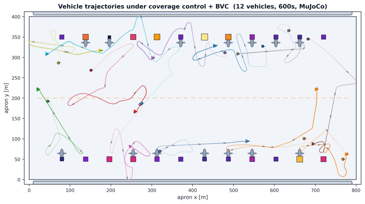
Trajectories confirm the coverage law working as intended: vehicles fan out from starting positions to cover both terminal rows, converging on demand-weighted centroids without colliding. The curving paths near busy gate clusters are not hand-coded; they emerge from the BVC projection deflecting each vehicle around its neighbors as they converge on the same region.
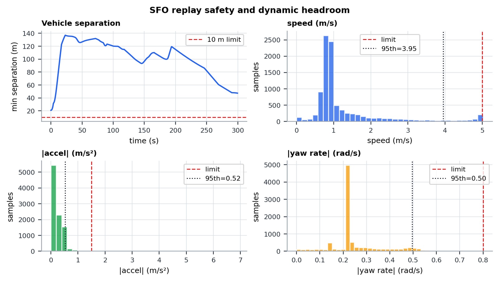
The safety headroom plots show the full 300-second, 16-vehicle replay. Minimum pairwise separation (top-left) starts near 20 m as vehicles fan out from clustered starting positions, grows to over 130 m at peak distribution, and stays above the 10 m safety radius throughout. The three histograms show that the fleet operates well within actuator limits in normal service; the 95th-percentile speed is 3.95 m/s against a 5 m/s cap, and 95th-percentile acceleration is 0.52 m/s² against a 1.5 m/s² limit.
| Metric | Value | Limit |
|---|---|---|
| Vehicle safety violations | 0 | 0 |
| Obstacle penetrations | 0 | 0 |
| Minimum vehicle separation | 31.6 m | > 10 m |
| Min gate / aircraft clearance | 0.750 m | > 0 |
| Max speed | 4.997 m/s | 5 m/s |
| 95th percentile acceleration | 0.242 m/s² | < 1.5 m/s² |
| Max yaw rate | 0.619 rad/s | 0.8 rad/s |
Extensions
Two higher-level analyses extend the base controller.
Worst-case demand game. The coverage cost is a function of both fleet positions and the demand distribution. If an adversary could allocate demand to maximally hurt coverage, concentrating it at the gates farthest from the current fleet configuration, what positioning would the fleet choose to stay robust? The minimax problem
is solved via best-response iteration: the fleet takes a Lloyd step, then an adversary reallocates demand toward the currently worst-served gates, and the process repeats. The resulting positions are more robust to unexpected demand spikes than the unconstrained Lloyd solution.
MAPPO extension. Lloyd’s algorithm is reactive; it responds to current demand but cannot anticipate future arrivals. A MAPPO policy replaces the centroid command with a learned action conditioned on each agent’s local observation (own state, neighbor positions, local gate demand, time features). A centralized critic uses fleet-level information during training but is not available at deployment. The BVC filter stays in the loop as a hard safety layer: the policy proposes, the QP clears it for collision.
Related projects
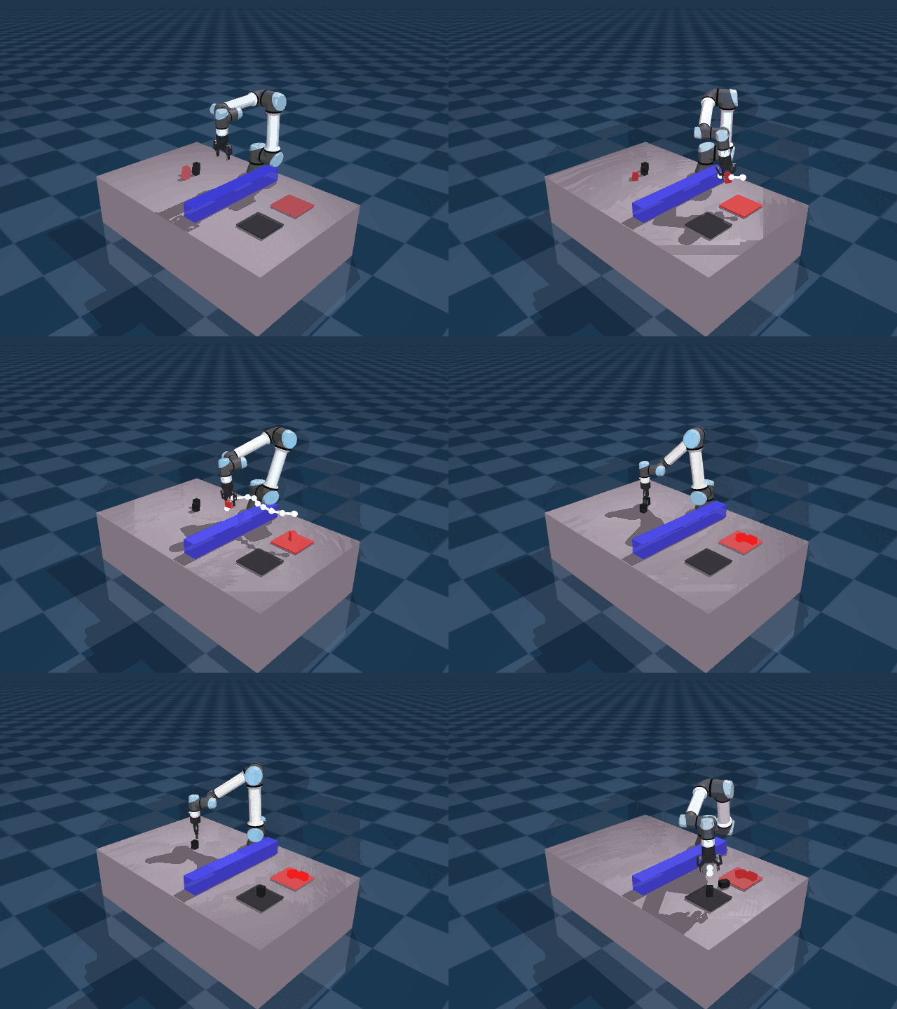
MPC for UR7e Robotic Arm: Warehouse Sorting
Constrained joint-space Model Predictive Control for a UR7e manipulator. An RGB-D perception pipeline localizes objects and obstacles; a receding-horizon CasADi/IPOPT solver generates collision-free joint trajectories at 12 Hz, validated in MuJoCo and deployed on real hardware.
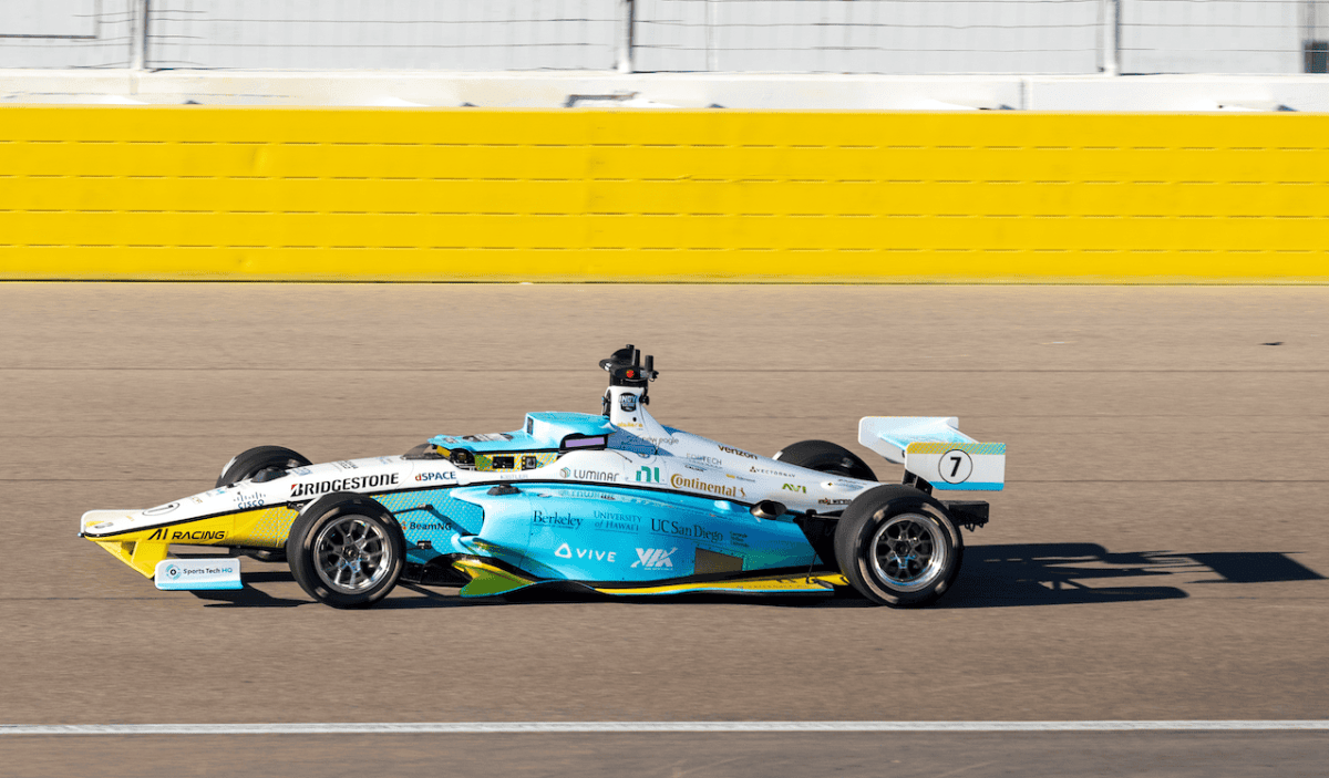
Nonlinear MPC for Autonomous Racing
Progress-maximizing NMPC for a full-scale Dallara AV-24 competing in the Indy Autonomous Challenge. Two-timescale architecture: a full-lap minimum-time NLP solved offline with a double-track Pacejka vehicle model produces the Track Trajectory Library, while an NMPC at 100 Hz in a Frenet frame executes it with RTI. Validated in AWSIM (best lap 117.6 s, 207 km/h max) and on the physical car.
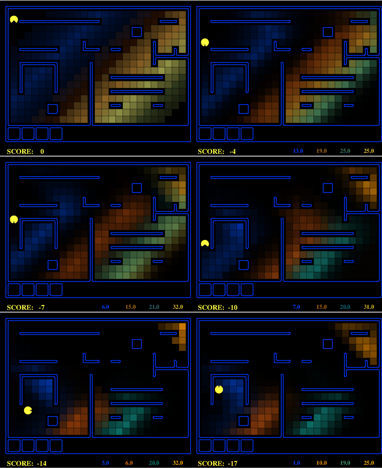
Pacman AI: A Tour of Classical AI
End-to-end AI agent built across four paradigms: A* pathfinding, Minimax/Expectimax game trees, HMM + particle filter tracking, and Q-learning. Each piece solves one Pacman problem; together they cover the full classical AI curriculum.