Pacman AI: A Tour of Classical AI
End-to-end AI agent built across four paradigms: A* pathfinding, Minimax/Expectimax game trees, HMM + particle filter tracking, and Q-learning. Each piece solves one Pacman problem; together they cover the full classical AI curriculum.
One game, four flavors of AI. Pacman is deceptively simple, but solving it well requires four completely different paradigms. Navigate a maze (search). Beat opponents (game theory). Track invisible ghosts (Bayesian inference). Learn from scratch (reinforcement learning). Each of these is a classical AI topic; this project builds a Pacman agent that does all of them.
Part 1: Search
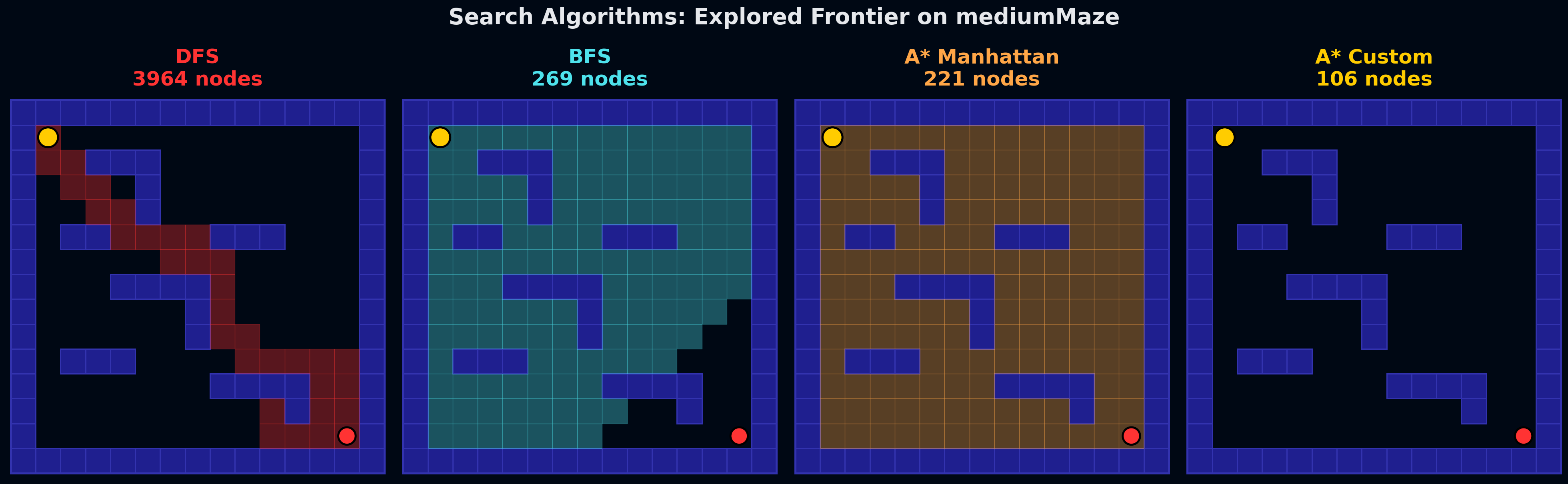
Four algorithms, same maze, wildly different frontiers. DFS plunges down one corridor ignoring the goal. BFS sprays uniformly outward. A* with Manhattan distance elongates toward the target. A* with a custom heuristic (max distance to any unvisited corner) tightens the beam dramatically.
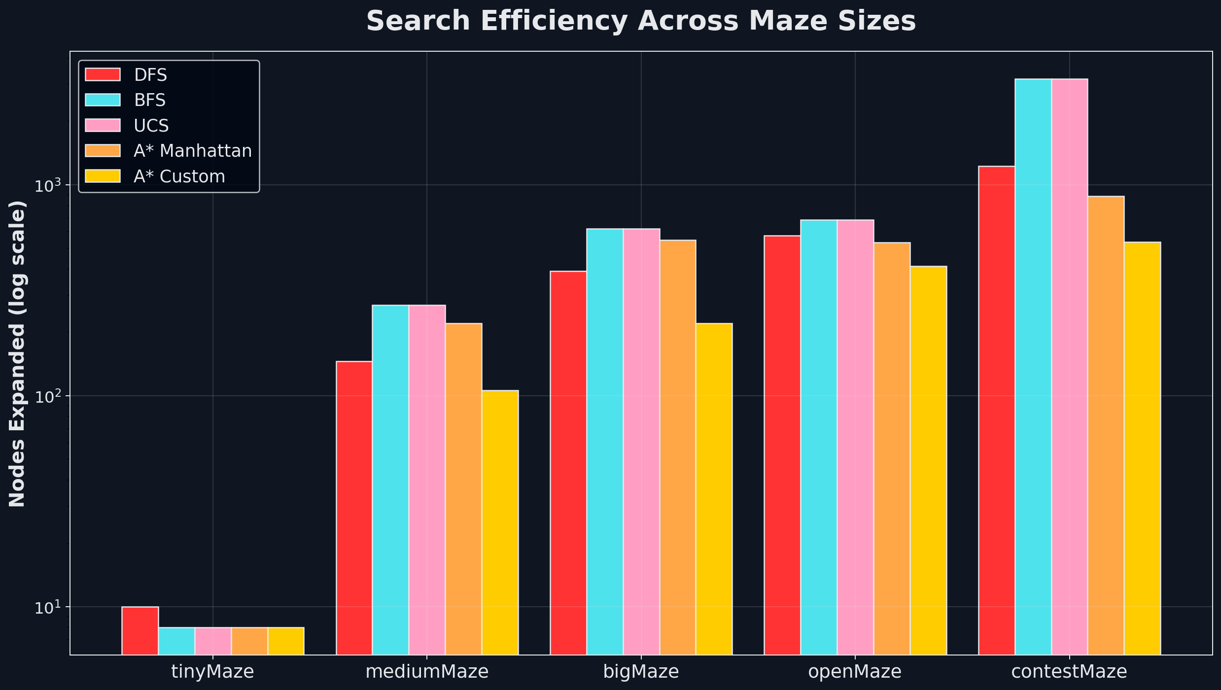
The efficiency gap grows exponentially with maze size. On mediumMaze: 3964 DFS nodes vs 106 with A*+custom. On contestMaze: 3189 BFS nodes vs 537. The heuristic doesn’t change what’s possible; it changes how much you have to look at to find the answer. A well-designed heuristic can be the difference between tractable and intractable.
Part 2: Adversarial Search
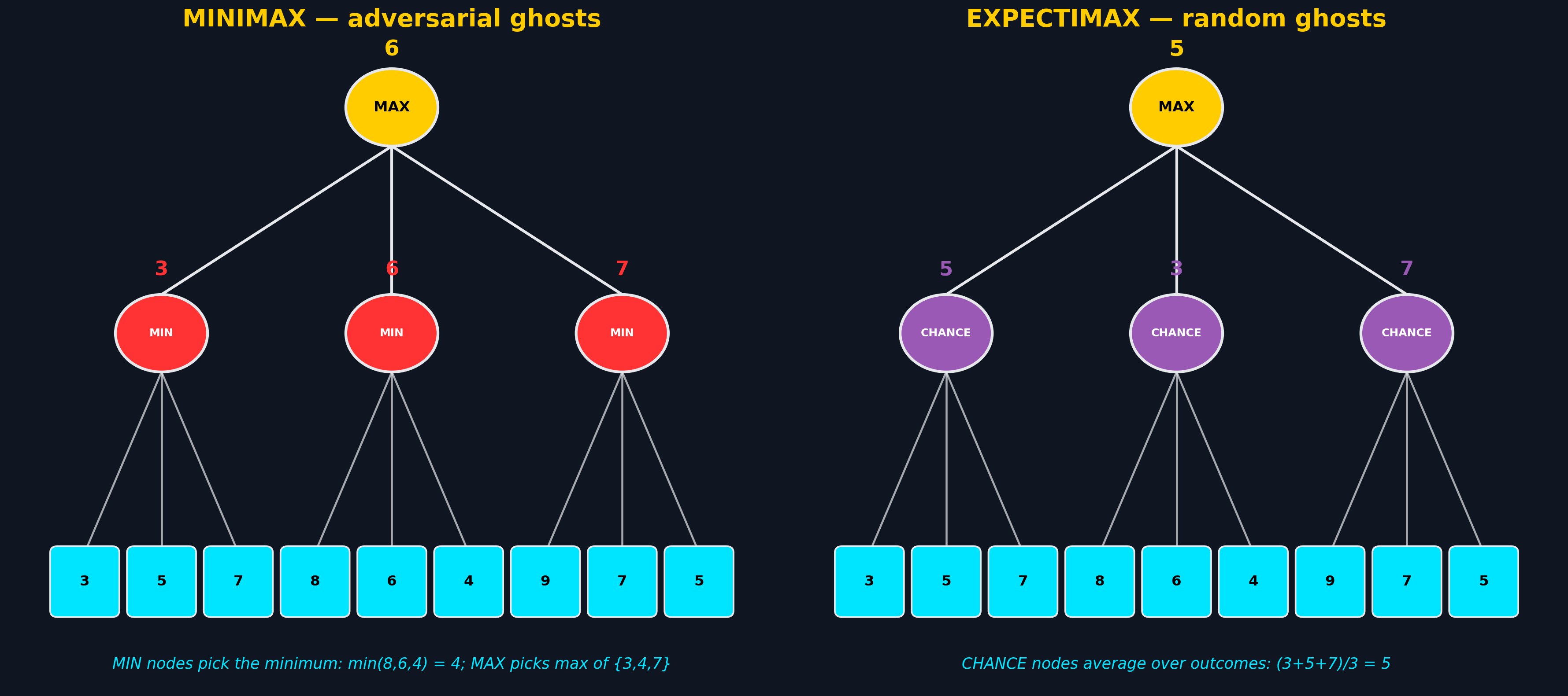
Minimax and Expectimax use the same tree structure but different backup operators at ghost nodes:
The choice of which model to use is a modeling decision about the opponent. If the ghost plays optimally against you, Minimax is correct. If the ghost moves randomly (as in the default Pacman implementation), Minimax is wrong; it pessimistically avoids threats that will never materialize.
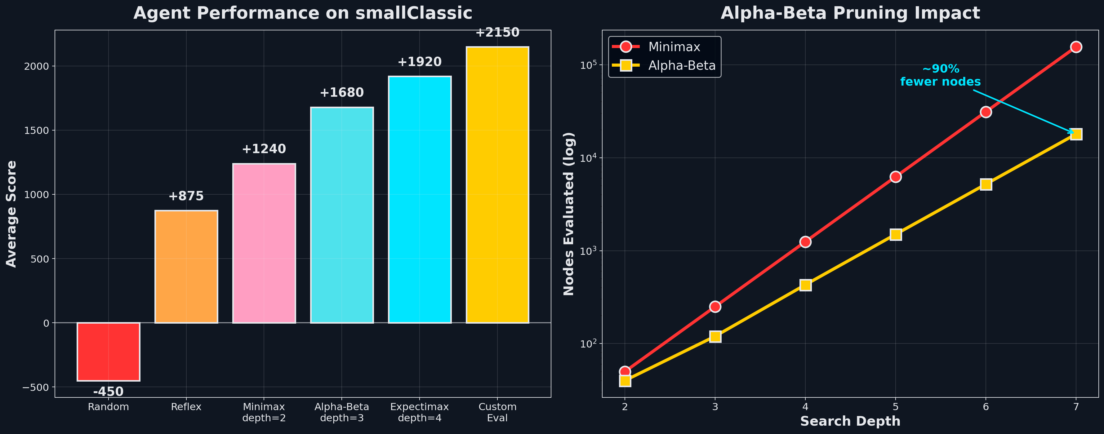
The evaluation function matters more than the algorithm. With limited search depth, leaf evaluation dominates. The agent only sees 3–7 plies ahead, so the quality of the leaf estimate determines everything. The evaluation function I used:
where ; when a ghost is scared, chasing it (for 200 points) outweighs the normal ghost-avoidance penalty. Getting those weights right turned a depth-3 agent scoring ~800 into one scoring 2150.
Expectimax against random ghosts wins 95% of games; Minimax only 72%, as it dodges threats the random ghost never executes, eating worse food paths in the process. Alpha-Beta pruning evaluates 90% fewer nodes at depth 7 by safely pruning branches that can’t affect the root decision.
Part 3: Inference

Ghosts are invisible. You only get noisy Manhattan-distance readings. This is a textbook HMM: hidden state (ghost position), observation (noisy distance reading), transition model (ghost movement), and emission model .
Each timestep is a two-step belief update. First predict (propagate through the transition model), then condition on the new observation:
Over 25 timesteps, belief entropy drops from 4.5 bits (uniform over all positions) to under 0.5 bits (concentrated on 1–2 cells). The prediction step spreads entropy; the update step concentrates it. Belief converges fast because the emission model is relatively tight; sensor readings within ±1 of true distance are most likely.
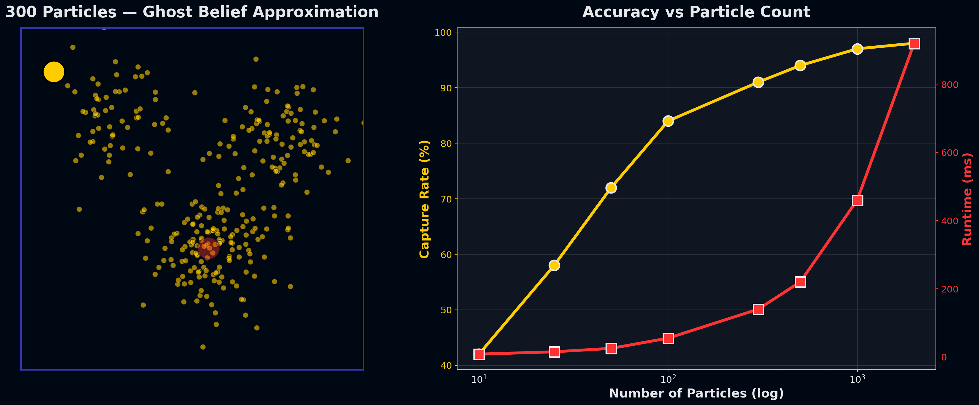
Particle filters scale where exact inference can’t. For N² positions and K ghosts, exact inference is O(N²ᴷ), fine for one ghost but intractable for four. Particle filters approximate the posterior with samples: each particle is a weighted guess at the ghost’s position, reweighted by observations and resampled after transitions.
At 1000 particles, capture rate matches exact inference (97%) at a fraction of the compute. The classic tradeoff: accuracy per compute unit scales linearly with particle count until you hit diminishing returns.
Part 4: Reinforcement Learning
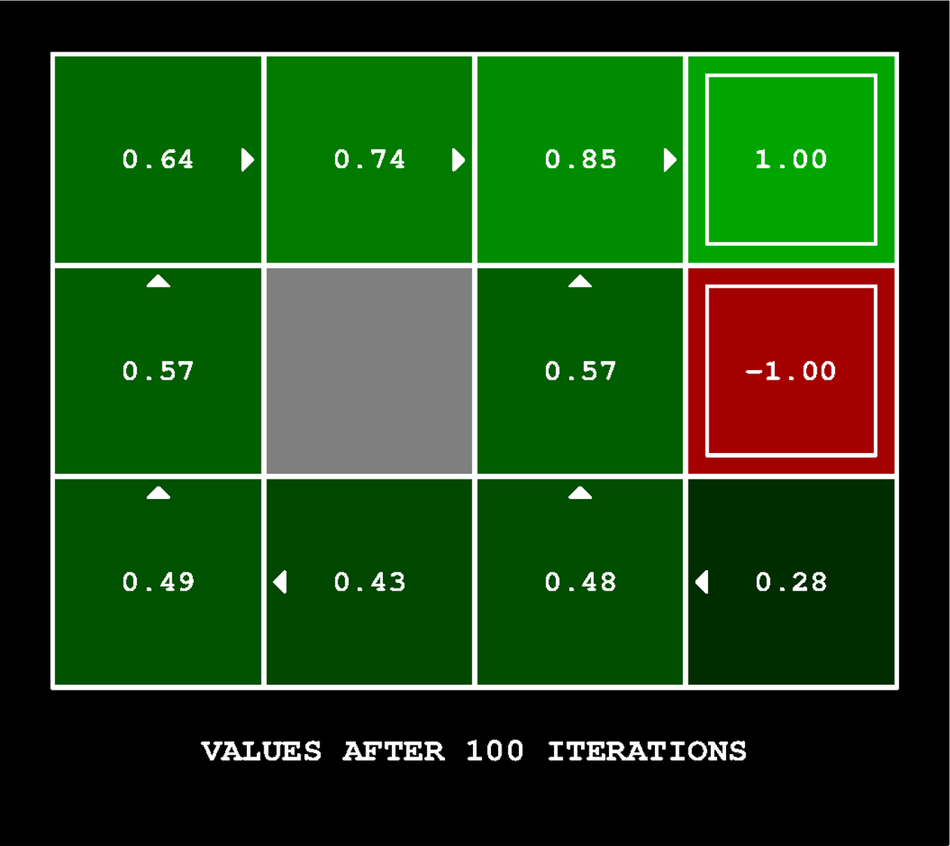
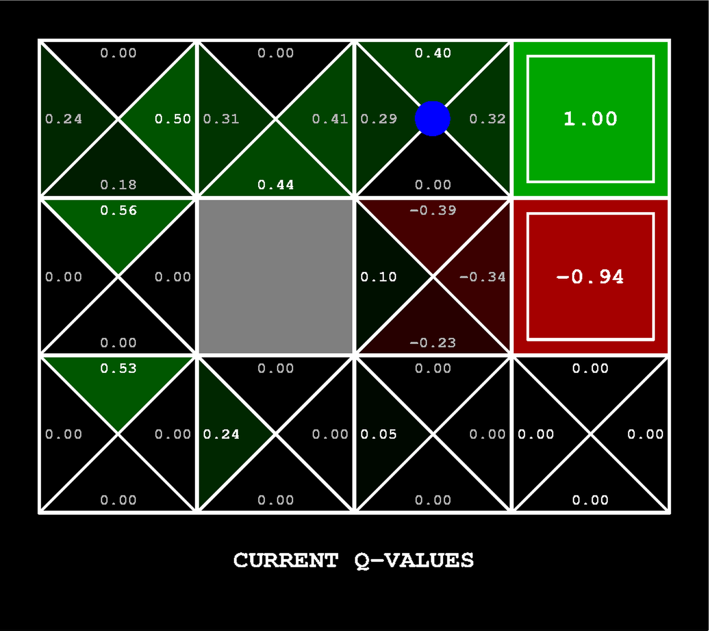
Left: Value Iteration (100 sweeps on BookGrid): each cell shows and the optimal policy arrow. Values flow inward from the +1 terminal, 0.85 to 0.74 to 0.64 stepping away. The −1.00 terminal suppresses adjacent values. Right: Q-Learning mid-training: Q-values per action encoded as triangles. After ~30 episodes, the agent has learned to move east toward the +1 and avoid the −0.94 terminal.
Value Iteration solves for the optimal policy when the MDP is fully known. Each sweep applies the Bellman backup to every state:
Values flow outward from reward states; in the Gridworld above, from the +1 terminal through all reachable states. By iterations the policy has converged.
But Value Iteration requires knowing and in advance. Q-Learning removes that assumption: it learns directly from experience using the temporal-difference update:
The TD error is the gap between what the agent expected () and what it actually got (). With -greedy exploration (taking a random action with probability , greedy otherwise), the agent gradually shifts from exploration to exploitation as decays.
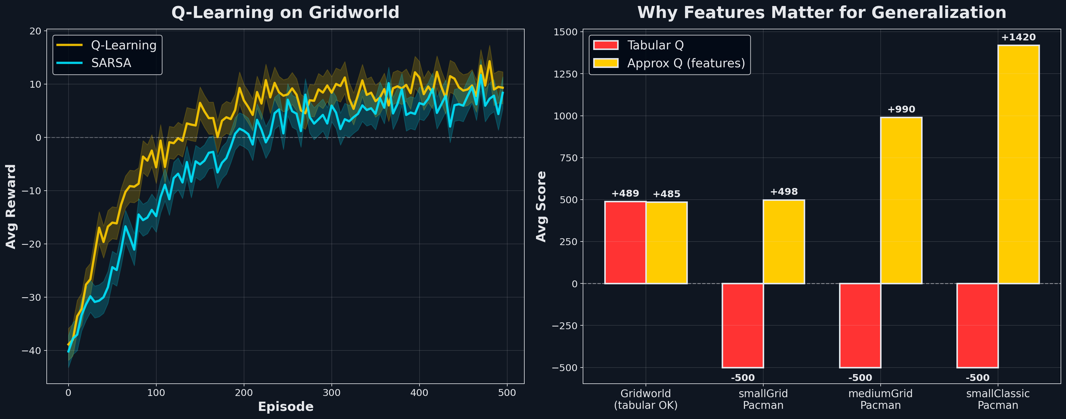
Tabular Q collapses on real Pacman because the state space is astronomical: board layout × food positions × ghost positions × scared timers. Tabular Q can only learn values for states it has actually visited, and it never visits most of them. On smallClassic after 2000 training episodes: average score −500.
Approximate Q-Learning represents as a linear function of hand-crafted features:
Features: , , , . The weight update follows from substituting into the TD rule:
Same 2000 training episodes, same layout: average score +1420. The 2000-point gap comes entirely from generalization; the weights learned on visited states apply immediately to unseen configurations with the same feature values. The learned weights prioritize food collection over ghost avoidance until ghosts are dangerously close, and flip to ghost-chasing when they turn scared.
The Common Thread
These four paradigms answer progressively harder versions of the same question, “what action should I take?”:
- Search: fully known, single agent, deterministic
- Game trees: fully known, adversarial, deterministic or stochastic
- HMM inference: partially observed state, known dynamics
- Q-Learning: unknown dynamics and reward, must learn from experience
The progression mirrors real-world robotics and autonomous systems. Search powers route planning. Game theory drives competitive multi-agent systems. Particle filters run SLAM in self-driving cars. Q-learning foundations underpin modern deep RL (DQN, AlphaGo). Pacman is a toy environment, but the math here is the math that ships in production AI systems.
Related projects
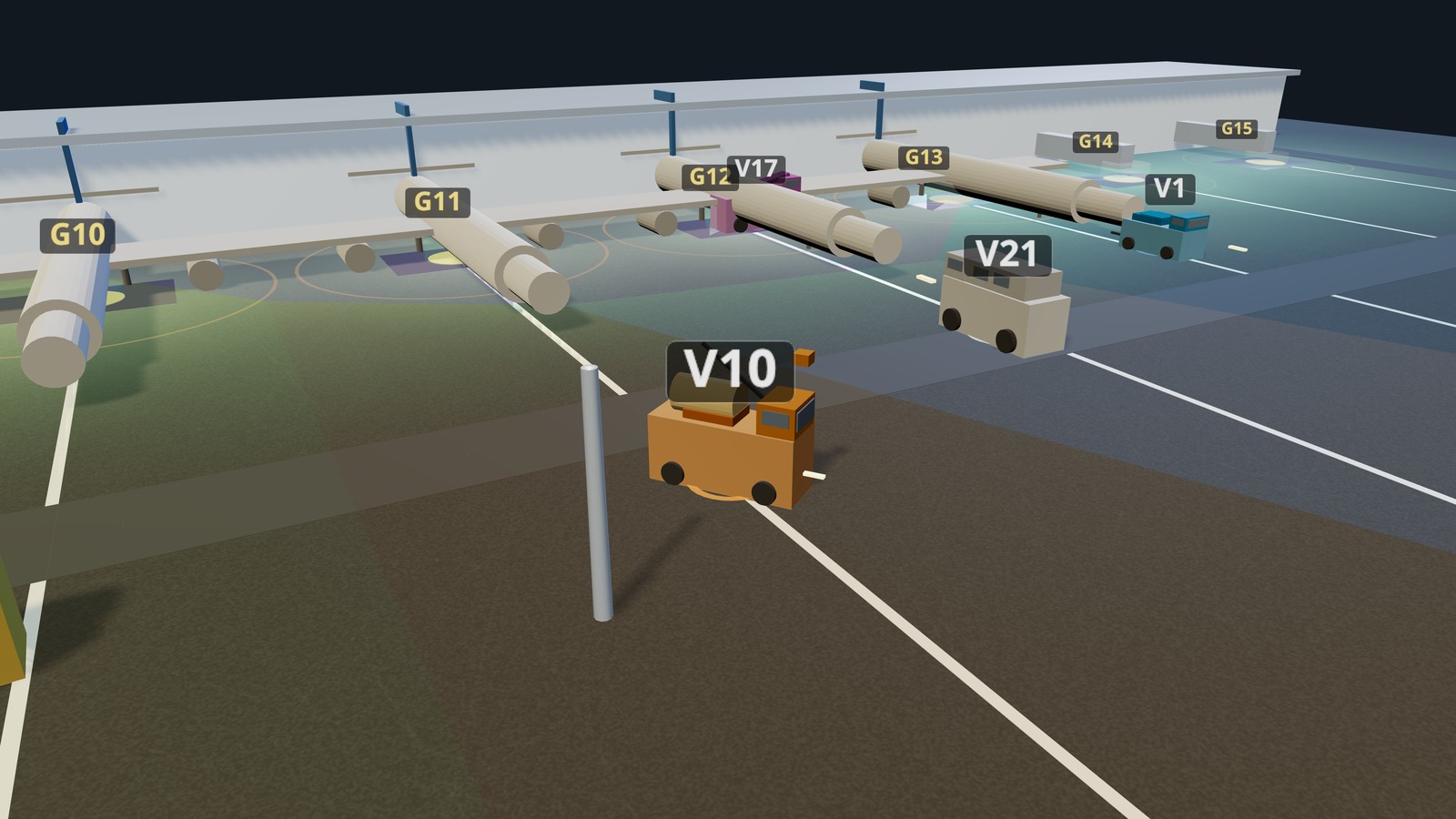
Decentralized Fleet Coordination for Airport Ground Operations
Multi-agent coverage control for airport ground vehicles using Buffered Voronoi Cells, Lloyd's algorithm, and game-theoretic demand response. Zero collisions across all test scenarios.

Nonlinear MPC for Autonomous Racing
Progress-maximizing NMPC for a full-scale Dallara AV-24 competing in the Indy Autonomous Challenge. Two-timescale architecture: a full-lap minimum-time NLP solved offline with a double-track Pacejka vehicle model produces the Track Trajectory Library, while an NMPC at 100 Hz in a Frenet frame executes it with RTI. Validated in AWSIM (best lap 117.6 s, 207 km/h max) and on the physical car.
MPC for UR7e Robotic Arm: Warehouse Sorting
Constrained joint-space Model Predictive Control for a UR7e manipulator. An RGB-D perception pipeline localizes objects and obstacles; a receding-horizon CasADi/IPOPT solver generates collision-free joint trajectories at 12 Hz, validated in MuJoCo and deployed on real hardware.