Deep Learning from Scratch
The full arc: backpropagation in raw NumPy, CNNs with BatchNorm and Dropout trained to 78% on CIFAR-10, multi-head self-attention for text summarization, and a Masked Autoencoder that reconstructs images from 25% of their patches, then transfers those features to downstream tasks.
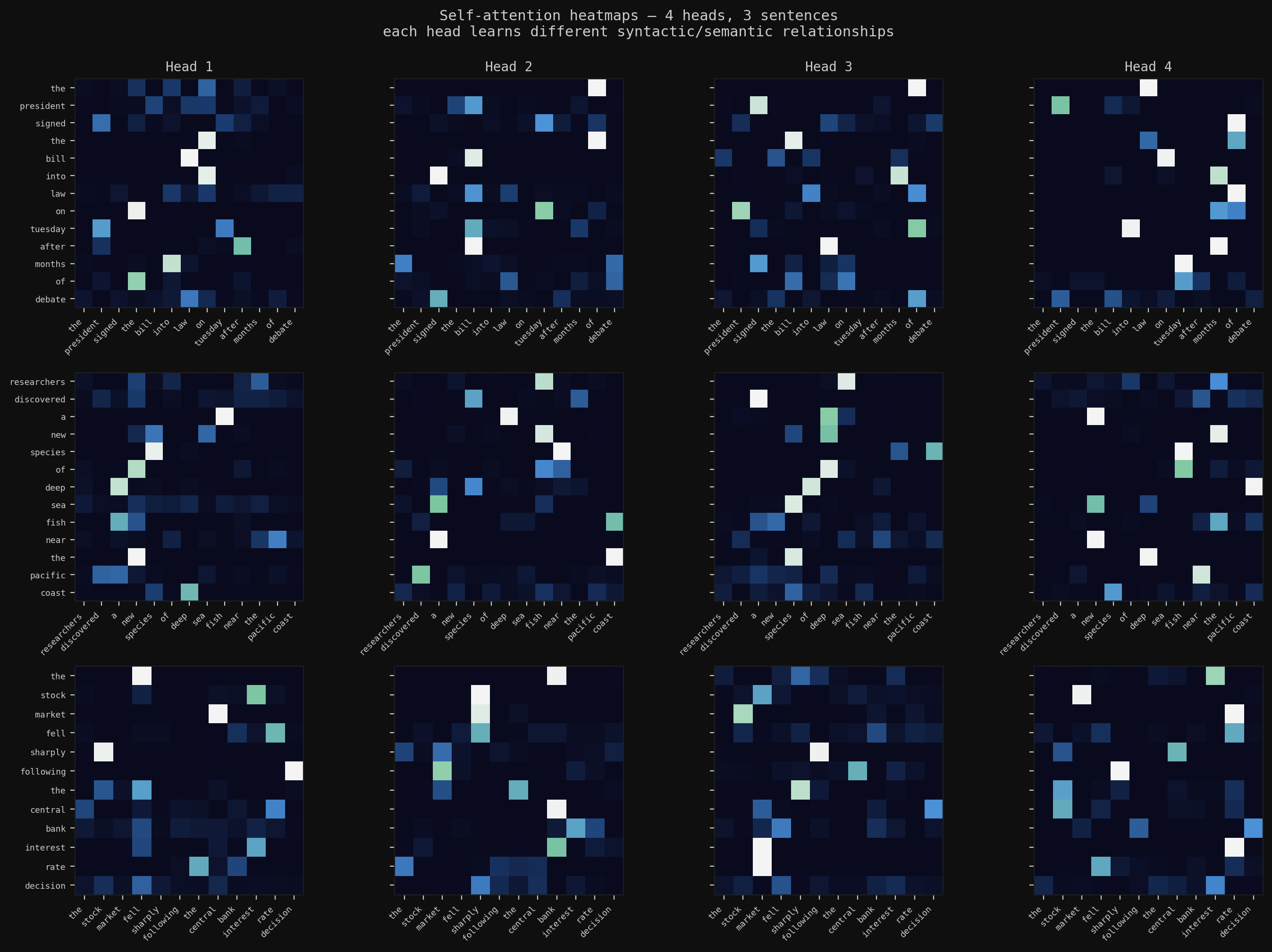
4 attention heads on 3 sentences, each head independently learning different relationships: syntactic structure, named entity routing, long-range dependencies. This project builds everything behind that from scratch: the forward pass in NumPy, CNNs with BatchNorm, the full attention mechanism, and a Masked Autoencoder for self-supervised pretraining.
Part 1: Backprop by Hand
Before touching PyTorch, the full forward and backward pass was written in NumPy: convolution as a loop over patches, pooling with argmax masks for gradient routing, softmax cross-entropy, and the chain rule applied manually through every layer. No autograd.
The goal was to feel where gradients actually go: which layers throttle them, what happens when activations are poorly conditioned, why depth alone doesn’t guarantee a trainable network.
Learned Filters
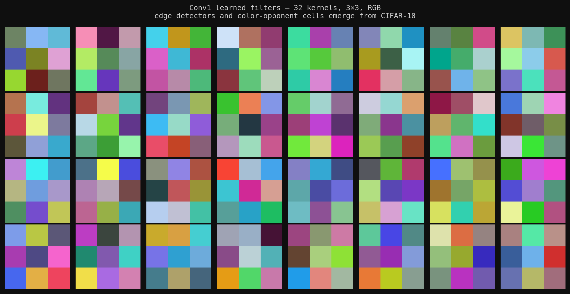
32 first-layer filters after training on CIFAR-10. Color-opponent pairs and oriented edge detectors emerge without being specified, the same structure Hubel and Wiesel found in V1 cortex, now arising from gradient descent on 50,000 photographs.
Part 2: BatchNorm, Dropout, and Why They Work
Same architecture (Conv32→Conv64→Conv128→FC256→FC10), trained with and without BatchNorm across a range of learning rates.
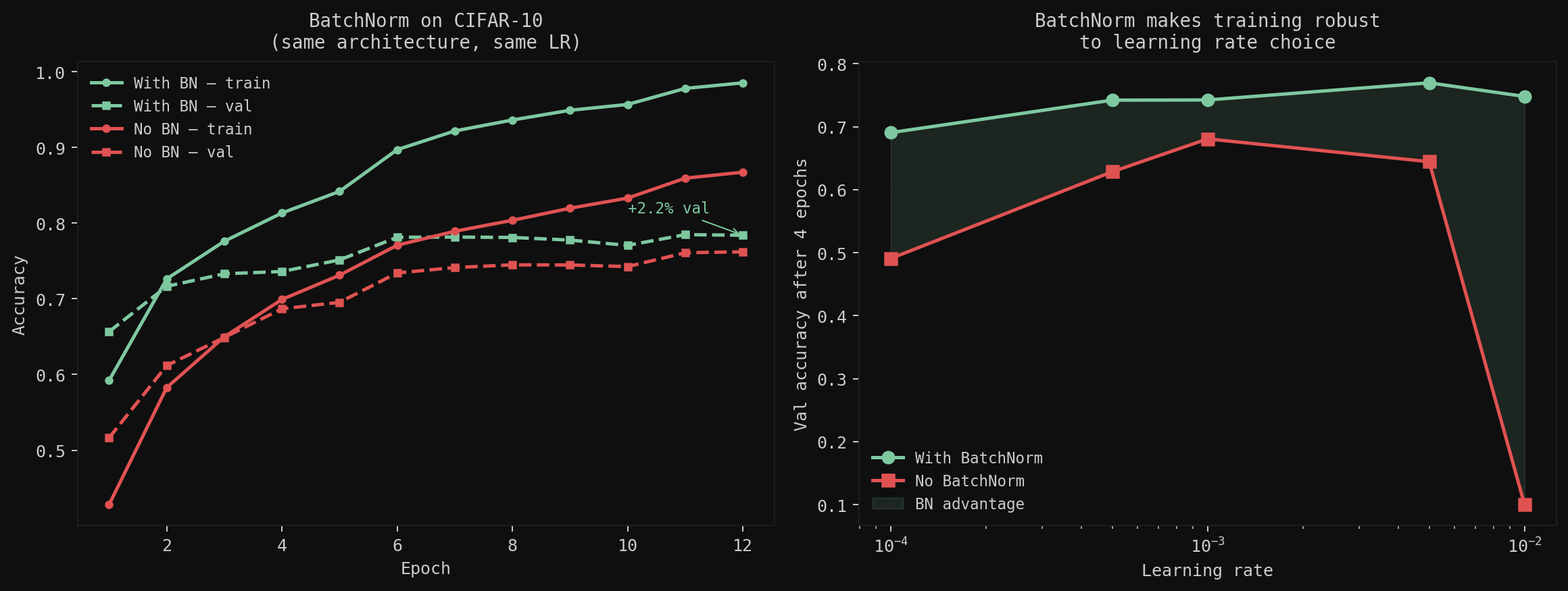
The LR sweep is the telling result. The BN model holds near-peak accuracy across a 100× range of learning rates. The plain model has a narrow sweet spot. That robustness, not the 2% accuracy bump, is why BatchNorm became standard.
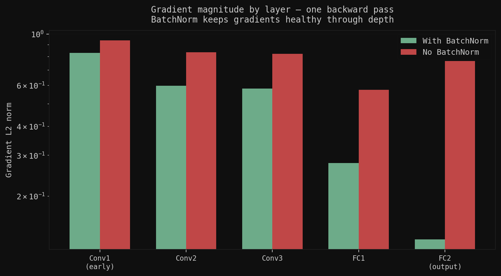
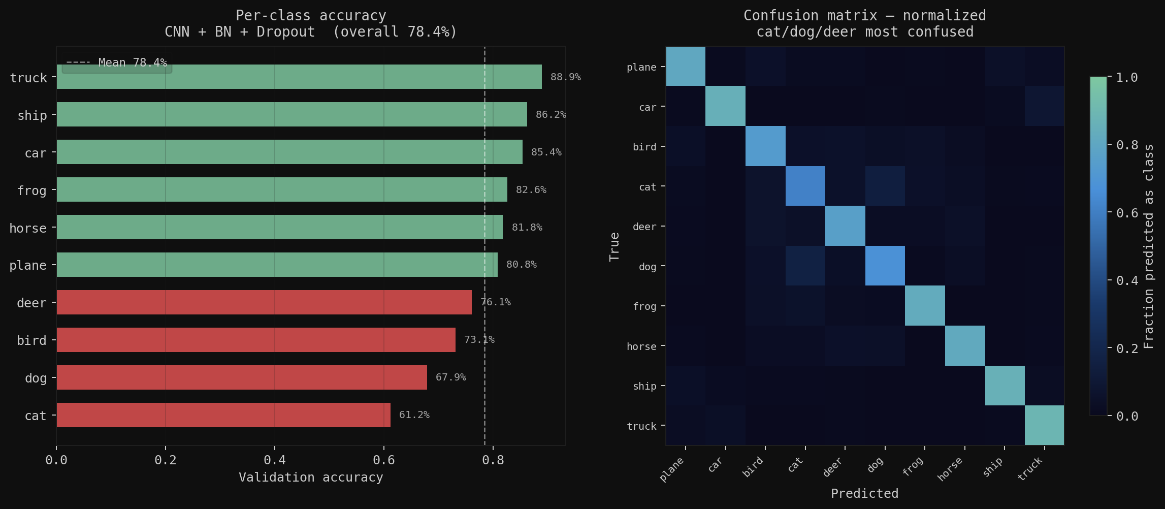
Left: gradient norms on one backward pass. Without BN, early layers get large uneven gradients. With BN, they stay consistent from FC2 back to Conv1. Right: final results, 78.4% overall. Trucks (88.9%) and ships (86.2%) are easy; cats (61.2%) are the hardest. The confusion matrix shows exactly where the model breaks: cat-dog is the single largest off-diagonal entry, two quadrupeds at similar scale and texture.
Part 3: Multi-Head Self-Attention
4 attention heads on 3 news sentences; no two heads are doing the same thing. One tracks syntactic structure (near-diagonal), one routes through named entities, one connects long-range dependencies. The multi-head structure lets each head specialize on different relationship types within the same sequence.
A full encoder-decoder Transformer was trained for news summarization: separate stacks, cross-attention in the decoder, sinusoidal positional encodings. Teacher forcing during training (feed the correct prefix, not the model’s own output) makes gradients sharp but creates a distribution gap at inference that beam search partially closes.
Part 4: Masked Autoencoder
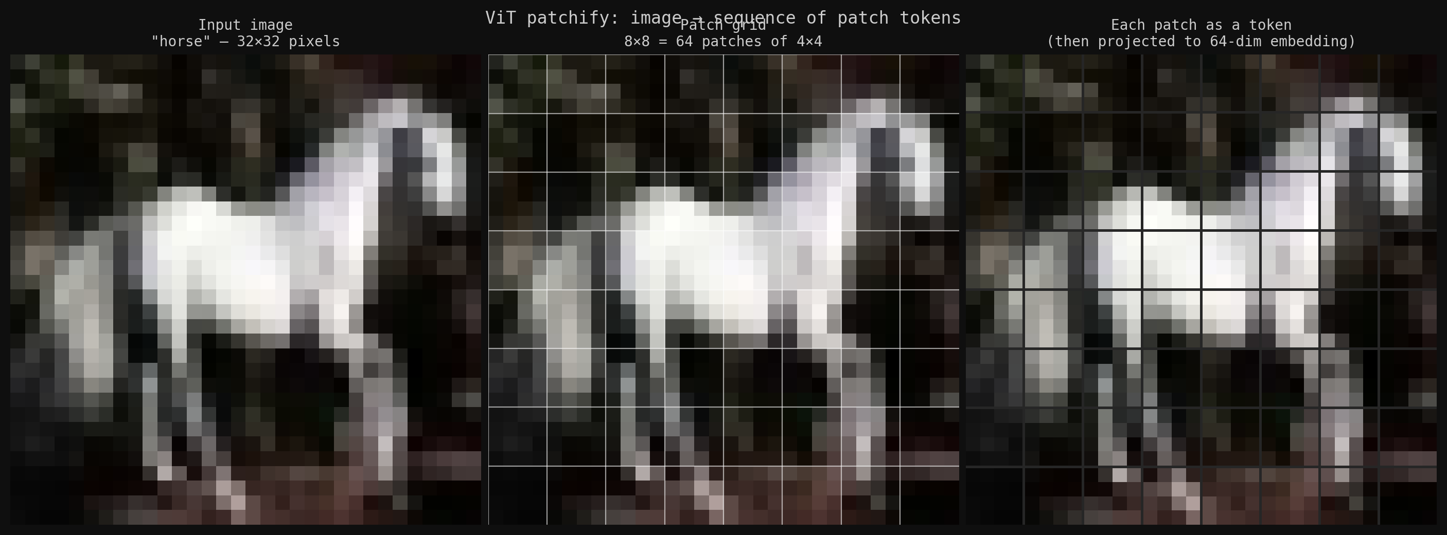
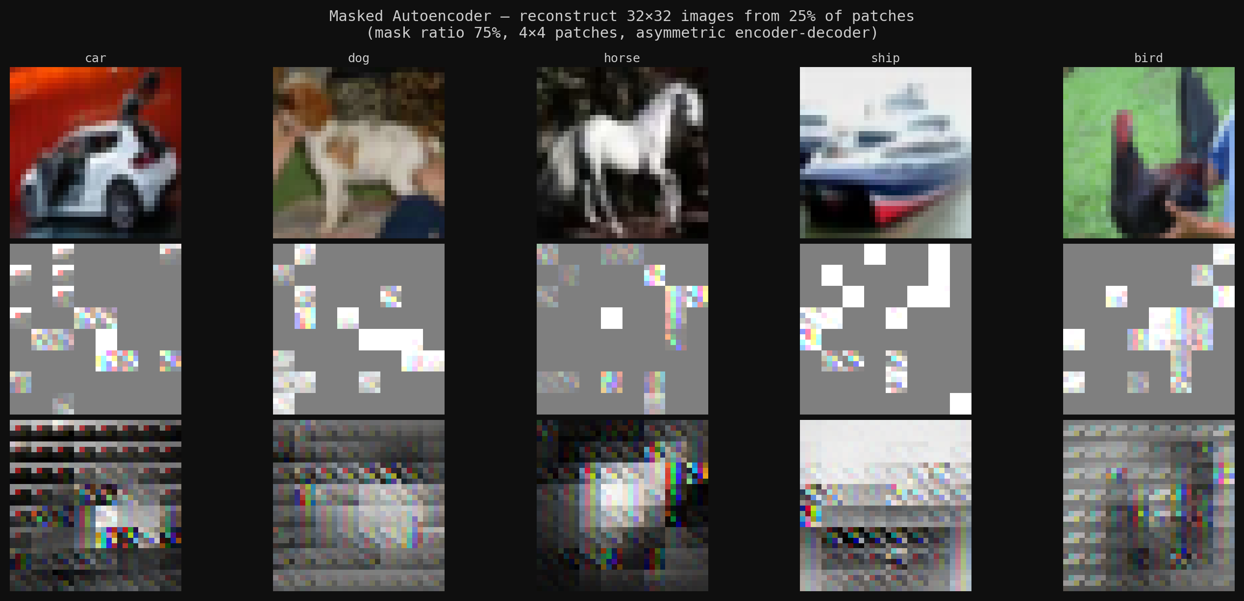
A 32×32 image is divided into 64 non-overlapping 4×4 patches, each linearly projected into a token, the same operation as a word embedding but for image regions. 75% of patches are then masked at random. Only the visible 25% pass through the encoder; the decoder reconstructs the missing pixels.
The asymmetry is the point: heavy masking prevents the model from just interpolating neighbors, so the encoder is forced to build globally coherent scene representations. The decoder is thrown away after pretraining.
Transfer
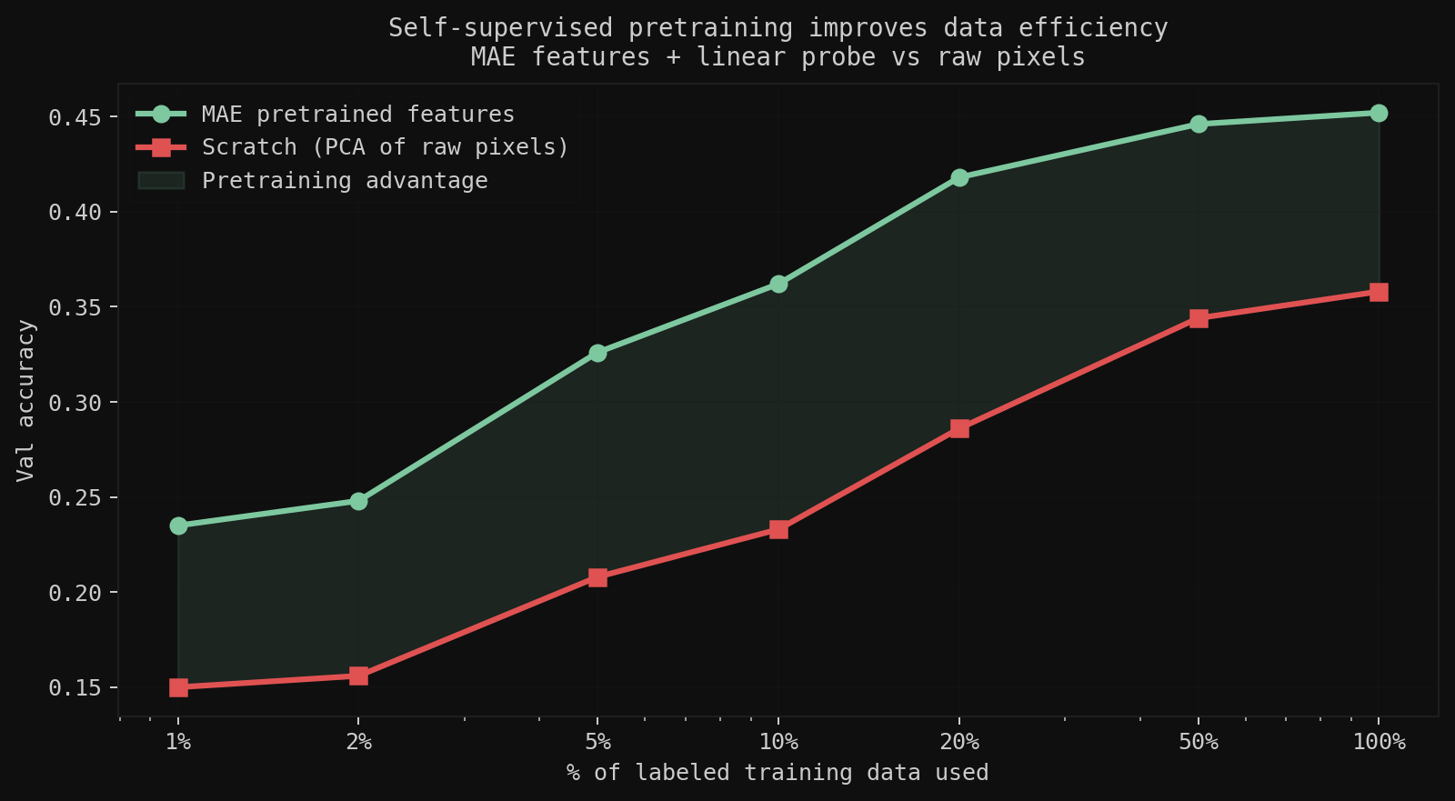
After pretraining on unlabeled CIFAR-10, the encoder is frozen and a single linear layer is trained on top. At 1% of labeled data (~500 images), the pretrained encoder is 57% more accurate than raw pixels. The gap shrinks as more labels are added; self-supervision is most valuable exactly when labeled data is scarce, which is most of the time in practice.
Related projects
Classical ML from Scratch
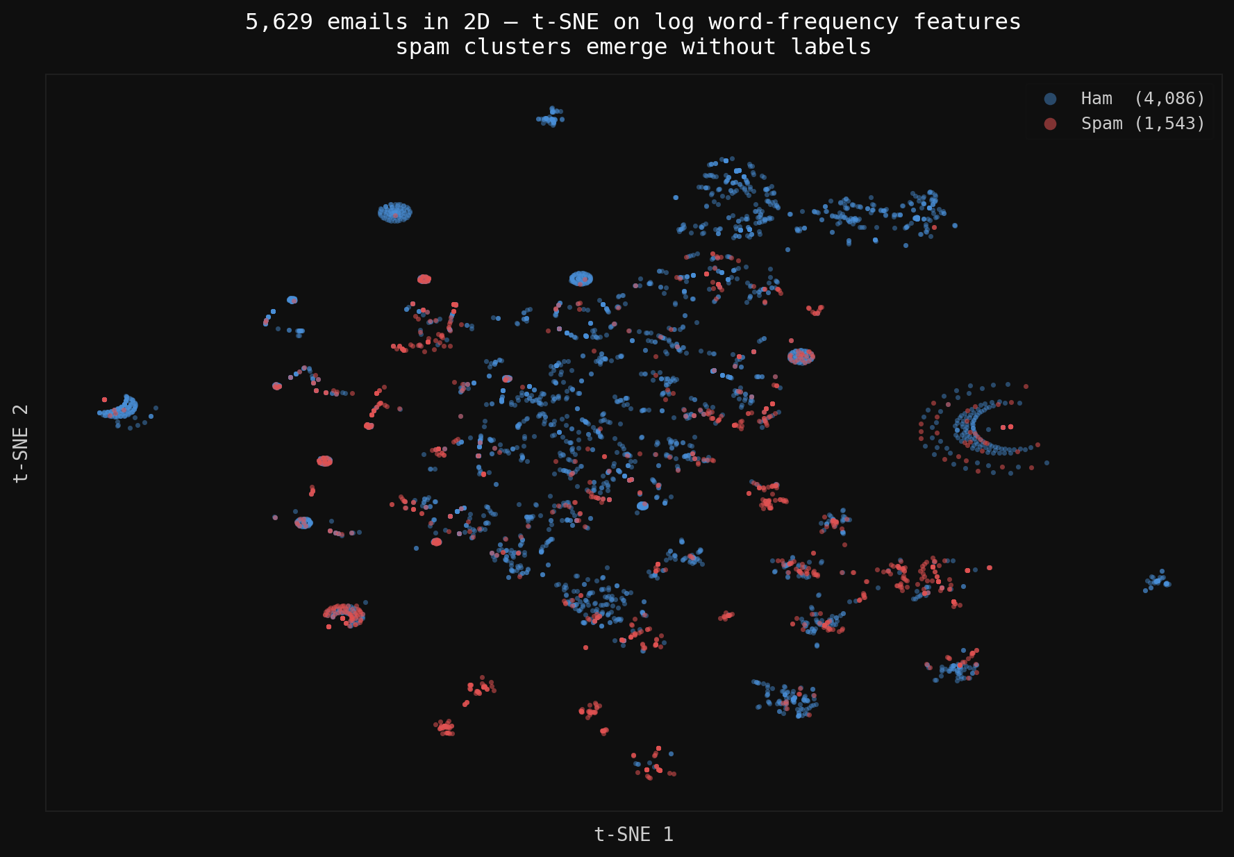
Two learning paradigms built from NumPy up: tree-based spam classification (decision tree, Random Forest, AdaBoost) and SVD/ALS matrix factorization for movie recommendations. No frameworks; matched scikit-learn on both.
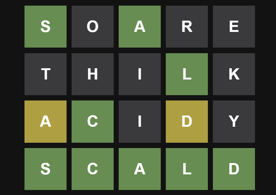
Entropy Wordle Solver
Information-theoretic greedy solver that picks each guess to maximize expected entropy over the remaining word set, averaging 3.92 guesses across 300+ games.
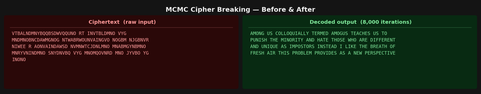
MCMC Cipher Decoder
Metropolis-Hastings breaking substitution ciphers against bigram frequencies. Watch garbled text slowly resolve into English over MCMC iterations.