An Autonomous Fleet Manager for 1,600 Satellites
Guidance, navigation, and control software that runs a constellation of electric propulsion satellites on its own. It keeps every satellite in its place in the formation, works out which close passes are real threats, and moves a satellite out of the way only when it has to. Designed around an eight mode state machine, tested in a simulated world full of errors the software is never told about, at the size of a full Starlink shell, and checked against CelesTrak's SOCRATES on the real satellite catalog.
This is guidance, navigation, and control software for a constellation of satellites in low Earth orbit. Each satellite has a single electric thruster that pushes with 25 millinewtons. The software keeps every satellite in its assigned place in the formation, finds out which passing objects are actually dangerous, and moves a satellite out of the way when one is. It does this for every satellite at once, with no operator involved.
I tested it in a simulated world that is harder than the software’s own picture of it. Every satellite has its own errors in drag, thrust, and thruster pointing, and the software is never told what they are. The film replays one run from its recorded data: 1,600 satellites, the size of one Starlink shell, flown for 12 hours with 12 objects deliberately placed on collision courses. I chose only the camera and the lighting.
The rest of this page explains the system behind it: what it has to do, how it is built, the states it reasons about, how each part works, and how it was verified.
1. What it has to do
The mission, from the design specification I wrote before any code: maintain the geometry of an electric propulsion fleet, detect close approaches under uncertainty, avoid collisions, and return every satellite to its slot afterwards. As requirements that can be measured:
- No collisions. Judged on the true trajectories, not on what the software predicted.
- Every avoided encounter ends below a probability of collision, counting every pass of the encounter.
- Every satellite stays in its slot. Correction starts when it is 2 km out and continues until it is within 300 m.
- After an avoidance, the satellite returns to within 1 km of its slot.
- Propellant is spent sparingly. Each satellite carries 50 kg of propellant, about 2.1 km/s of velocity change. Avoidance should cost centimetres per second, and station keeping a small fraction of the total.
- No unsafe command is ever flown. A burn that fails a check, or a risk the software cannot fix, puts the satellite in a safe mode that only the ground can clear.
- Faster than real time at the scale of a full shell.
The thresholds are demonstration values chosen for the study, not any operator’s real ones. Section 6 checks each requirement against the results.
2. Architecture
5 m noise, every 120 s
start, duration, direction
The system has two halves, and the boundary between them is strict. The simulated world on the left is the truth: it moves every satellite with its hidden errors and logs every real close approach. The flight software on the right never reads it. It receives position measurements with 5 m of noise every two minutes, and it plans with a clean model that assumes no errors. The only thing that crosses back is a burn command (start time, duration, and direction), which the world then flies with the satellite’s hidden thrust and pointing error.
That boundary is what makes the results mean something. A controller tested against its own model always looks good. Every number on this page is measured in the simulated world.
Inside the flight software, each satellite runs the same chain on a two minute cycle: estimate where everything is, decide what this satellite is allowed to do, compute the thrust for that, check it, and send it. Screening for close approaches runs every hour and looks 24 hours ahead.
3. States and modes
The software reasons about five kinds of state. Each is kept in the coordinate frame that suits its job, because no single frame suits them all.
| State | What it holds | Frame | Why that frame |
|---|---|---|---|
| Truth state | position, velocity, mass: | inertial (ECI) | where the equations of motion are simplest; only the simulated world has it |
| Navigation state | the estimate and its uncertainty | inertial (ECI) | what the filter produces, for the satellite and every tracked object |
| Slot error | six relative orbital elements : size, phase, shape, and tilt of the orbit relative to the slot | relative elements | each one maps to one physical correction, so the controller can act on them separately |
| Burn command | start time, duration, direction | radial, along track, cross track (RTN) | directions that mean something to the spacecraft: up, forward, sideways |
| Conjunction state | time of closest approach, predicted miss, its uncertainty, probability of collision | encounter plane | the plane perpendicular to the relative velocity, where a pass becomes a 2D question: does the miss land inside the collision circle? |
On top of these, each satellite is in exactly one of eight modes, and the mode decides what it may do. The next mode is a pure function of the current mode and one set of observations (slot error, worst probability of collision, whether a plan is ready, whether the burn is done, whether closest approach has passed), so every transition can be tested on its own without running a simulation.
Three rules shape the machine. Collision risk outranks formation. A satellite keeping its slot stops slot control the moment a risky pass appears, because every slot burn would move the geometry the risk was computed for. An encounter is a series of passes. Two crossing orbits with nearly the same period meet every orbit, so a plan is judged by its worst pass, and the satellite only enters RECOVERY after the last one. SAFE is absorbing. It means the software has run out of options it trusts, and leaving it is a decision for the ground.
The complete transition table:
| From | To | When |
|---|---|---|
| NOMINAL | STATION_KEEP | slot error above 2 km |
| STATION_KEEP | NOMINAL | slot error below 300 m |
| NOMINAL, STATION_KEEP, RECOVERY | CONJUNCTION_WATCH | probability of collision at or above |
| NOMINAL, STATION_KEEP, RECOVERY, WATCH | CA_PLANNING | at or above , or at or above within 3 hours of closest approach |
| CONJUNCTION_WATCH | NOMINAL | back below |
| CA_PLANNING | CA_BURN | a burn passed validation |
| CA_PLANNING | CONJUNCTION_WATCH | no plan found, risk below |
| CA_PLANNING | NOMINAL | the risk dropped below while planning |
| CA_BURN | POST_CA_COAST | the burn finished |
| POST_CA_COAST | CA_PLANNING | risk still above , or above with time for another burn |
| POST_CA_COAST | RECOVERY | the last pass of the encounter is behind |
| RECOVERY | NOMINAL | slot error below 1 km |
| any | SAFE | a command failed validation, or risk above with no workable plan |
The 3 hour rule exists because of how probability of collision behaves near a decision. When the predicted miss is a few standard deviations away, the probability swings by orders of magnitude with ordinary estimate drift, and it can cross minutes before closest approach, when it is too late to act. Acting on watch level risk once the deadline arrives raised the fraction of safely resolved encounters in Monte Carlo from 0.68 to 0.85, before the Kalman filter was added.
4. Subsystems
Each part of the flight software is described the same way: its job, what goes in and out, the design and why, and how it was checked.
4.1 Dynamics
- Job
- Predict how any object moves, for both the simulated world and the flight software.
- In
- a state and a time span; for the world, the hidden errors
- Out
- the state at any later time, and how small errors grow along the way
- Verified by
- energy and Kepler's laws, the closed form J2 drift of the orbit plane, drag decay, the rocket equation, worked examples from Curtis and Vallado
Every object moves under Earth’s gravity, the extra pull of Earth’s equatorial bulge (the term), atmospheric drag, and its own thrust:
Here is the air density at altitude , the ballistic coefficient (mass per unit of drag area, so a larger means less drag), the velocity relative to the rotating atmosphere, and the commanded thrust. The three hidden errors are drawn separately for every satellite: density scaled by , thrust off by , thruster misaligned by . The flight software assumes all three are zero. Drag matters most: density in the upper atmosphere changes by about ten times with solar activity, so a model that is off by 50% is normal.
I rebuilt this propagator from de Ruiter’s Spacecraft Dynamics and Control one chapter at a time, and checked each piece against a known answer before building on it.
4.2 Navigation
- Job
- Know where this satellite and every tracked object are, and how sure that knowledge is.
- In
- position measurements, 5 m noise for our satellites and 10 m for tracked objects; the burns this satellite commanded
- Out
- estimated orbit and its uncertainty, for every object
- Verified by
- the reported uncertainty matches the actual errors (normalised error squared about 6 for 6 states), including through a burn with hidden thrust error
- Meets
- requirements 1 and 2
Each object is tracked by an extended Kalman filter that predicts with the flight model, including the burns the satellite itself commanded, and corrects with each measurement:
describes how a small error grows between measurements, computed from the derivatives of the force model. accounts for what the model leaves out, mostly the unknown drag. picks the position out of the state, and is the measurement noise.
The filter was not in the first version, and it is there because requirement 2 failed without it. With raw measurements the fleet is unsure of each satellite’s height by about 10 m. At that level a pass at 3 m and a pass at 25 m look almost equally risky, so the fleet burned for nearly everything and still left some passes above .
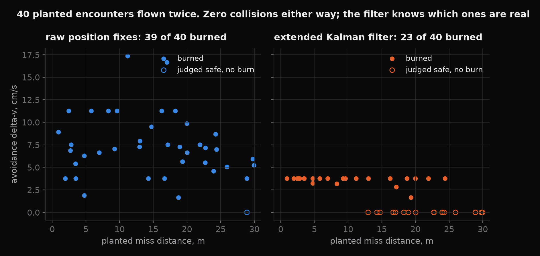
The same 40 random encounters (planted miss 0 to 30 m, crossing angles 30° to 150°, hidden errors), flown twice. Neither version collides, but only the filter meets requirement 2: every encounter ends below 10⁻⁶ (0.925 of them without it). It recognizes 17 passes as safe and leaves them alone, and spends half the propellant per avoidance, 3.6 cm/s against 7.4.
4.3 Station keeping
- Job
- Hold each satellite in its slot against drag.
- In
- slot error (relative elements), filtered over 30 minutes
- Out
- a thrust acceleration, recomputed every two minutes
- Verified by
- 96 satellites for three days with hidden errors; the 79 displaced satellites of the 1,600 satellite run
- Meets
- requirements 3 and 4
The key fact is that a higher orbit is a slower orbit. Let be how far the satellite is ahead of its slot along its path, how much larger its orbit is than the slot’s, the orbital rate, and the thrust acceleration along the direction of travel. The orbit equations give
Pushing forward raises the orbit, which slows the satellite and makes it fall back. So the along track error behaves like a mass pushed by a force, the same control problem as turning a rigid body with a torque. Drag acts on it like a constant force, and a controller that reacts only to the error and its rate (PD) settles with a steady offset under a constant force, so the law has an integral term:
The gains come from one requirement, a 2% settling time of one day with damping , by placing the closed loop poles there.
Three details made it work in practice. The thruster is weak, so a satellite far from its slot cannot be told to drift back quickly, or it overshoots. Without a limit, a 200 km correction overshot by 150 km. The controller therefore caps the drift rate it asks for at what half the thruster can stop, , and pauses the integral while the thruster is at its limit. The rate comes from through the equation above, not from differentiating noisy measurements. And the slot error that triggers the mode change weights the size error by the drift it will cause over 90 minutes, because a satellite can sit at the right place while drifting away at hundreds of metres an hour. Tilt and shape errors are corrected separately, by switching the thrust direction at the right points around the orbit.
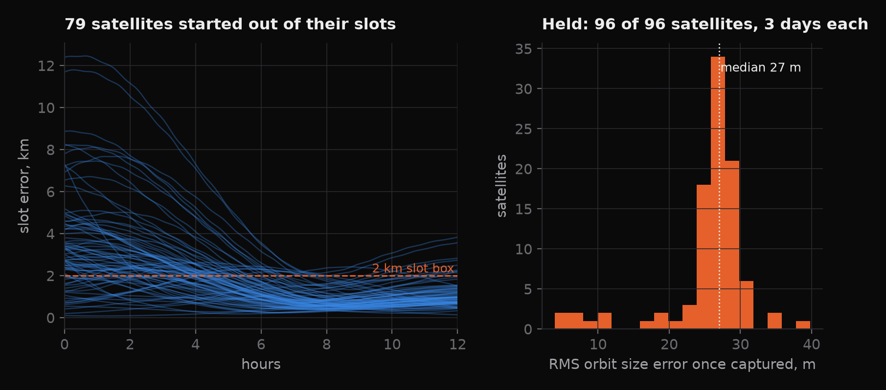
Left: the 79 satellites that started out of their slots in the 1,600 satellite run, some by 12 km. Most are inside the 2 km box by hour seven, and in the 48 hour run 77 of the 79 are back. Right: 96 satellites flown for three days, each with its own hidden errors. All 96 are captured and held, with a typical orbit size error of 27 m.
4.4 Conjunction assessment
- Job
- Find every close pass in the next 24 hours and say how likely each one is to be a collision.
- In
- estimated orbits and uncertainties of this satellite and every tracked object
- Out
- for each pass: time of closest approach, predicted miss, probability of collision
- Verified by
- closest approach times and misses reproduce SOCRATES within 0.5 ms and 0.5 m; probabilities agree between two independent methods
- Meets
- requirements 1 and 2
Screening samples every object’s position every 20 seconds and keeps every pass that comes within 5 km. At 20 second samples a pass at 9 km/s falls about 90 km from every sample, so each pass is resolved between samples by assuming straight line motion. Without that step, a 12 m encounter was invisible. Each pass is then refined to its exact time of closest approach, and both objects’ uncertainties are carried to that time and projected onto the encounter plane.
The probability of collision is the chance that the true relative position lands inside the 5 m circle formed by the two objects’ combined size, given the predicted miss and its uncertainty :
This is Foster’s method, checked against Alfano’s, an independent way of computing the same number. One refinement matters: a large uncertainty can make a dangerous pass look safe, because the probability is spread thin over a wide area. So decisions use the largest probability the pass could have as tracking improves, not today’s value.
4.5 Avoidance planning
- Job
- Find the cheapest burn that makes an encounter safe, early enough to check it worked.
- In
- the encounter's passes, their uncertainties, the satellite's mass and limits
- Out
- one burn command (start, duration, direction), or no plan
- Verified by
- 40 random encounters with hidden errors; the end to end acceptance test
- Meets
- requirements 1, 2 and 5
Risk is a hard constraint, not a term traded against fuel:
where is the burn’s centre time, duration, and one of six directions (up, down, forward, back, and both sides), and is the slot error the burn leaves for recovery to undo. The planner works in three steps:
- Score 90 candidates cheaply. Five lead times, three durations, six directions. Each is scored with the Clohessy–Wiltshire equations, which predict how far a short burn moves the satellite by closest approach, at the cost of one small matrix product instead of a full propagation.
- Verify the best few properly. The cheapest candidates that the prediction says will work are flown through the full flight model, closest approach is refined again, and the probability is recomputed against every pass of the encounter.
- Shrink the winner. Its duration is cut by bisection to the shortest burn that still meets the target.
Plans aim 100 times below the target, at , because they are made hours ahead on a wide uncertainty and checked later on a sharp one. Burns that end at least 90 minutes before closest approach are preferred, so the result can be measured from new measurements and corrected if it fell short. A burn whose result can only be checked when it is too late is a bet, not a plan. Before any burn flies it passes command validation: the duration and thrust are within limits, the satellite keeps more than its dry mass, and the burn actually lowers the risk. A failure sends the satellite to SAFE.
4.6 Attitude
- Job
- Point the body-fixed thruster in the burn direction before the burn, and hold it there.
- In
- the burn direction; the spacecraft's nominal mass properties
- Out
- reaction wheel torques
- Verified by
- a half turn flown on a spacecraft with 15% hidden inertia error and gravity gradient torque; stable from any starting orientation
- Meets
- requirement 2
The thruster is fixed to the body and normally points along the direction of travel, so a forward burn needs no turn. Every other direction does: a quarter turn to push up, down, or sideways, and a half turn to push backwards. Reaction wheels turn the spacecraft using quaternion feedback, a torque proportional to the attitude error and the rotation rate :
The flight software plans how long each turn takes from nominal mass properties, and the planner drops any candidate burn that would start before the turn has settled for 60 seconds. The simulated spacecraft then flies the turn with its true inertia, and the burn is fired along the axis it actually holds.
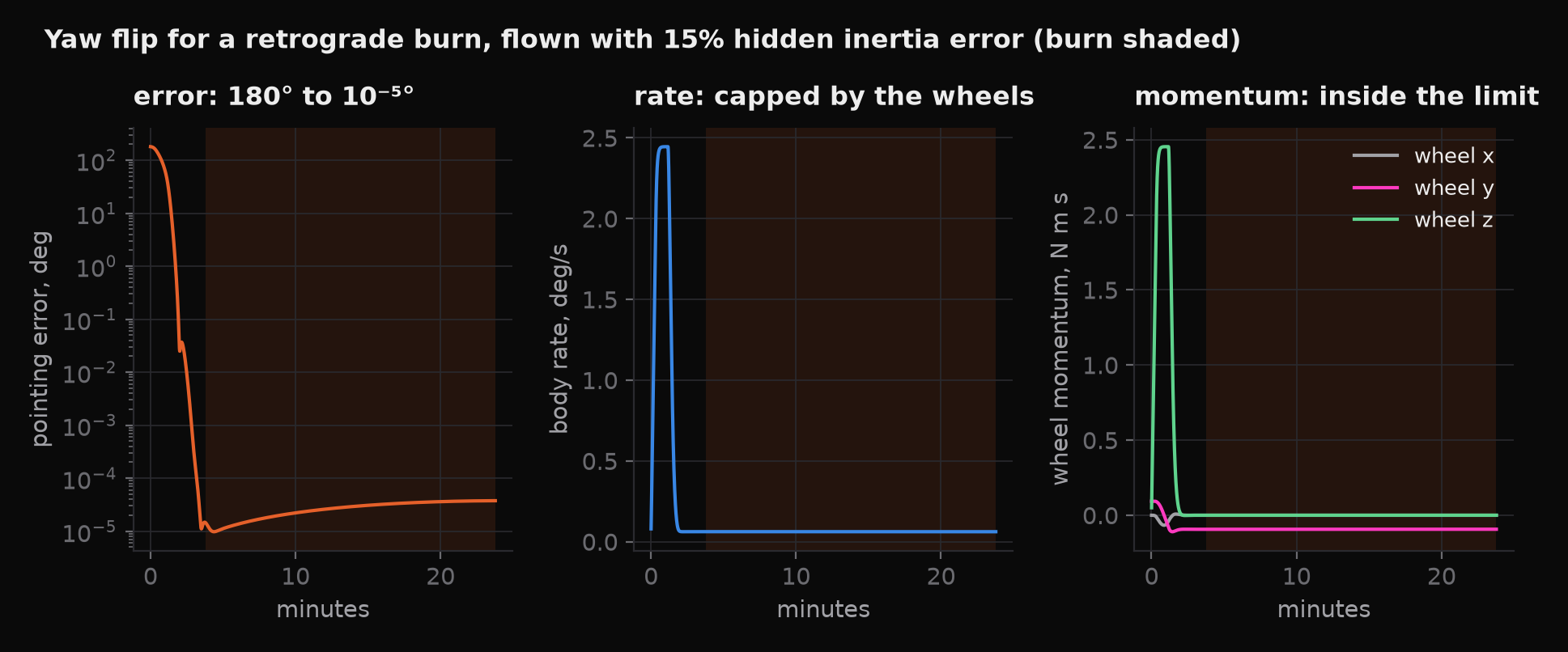
The half turn: the wheels apply their maximum torque, the spacecraft turns at the 2.4°/s the wheels can absorb, settles in about two minutes, and holds the thruster within about 10⁻⁵ degrees through a 20 minute burn.
5. One encounter, mode by mode
This is the pass from the film, traced through the state machine. The object was aimed to pass P47-S20 at 0.77 m, a direct hit. Press Replay P47-S20 on the state machine above to step through the same history.
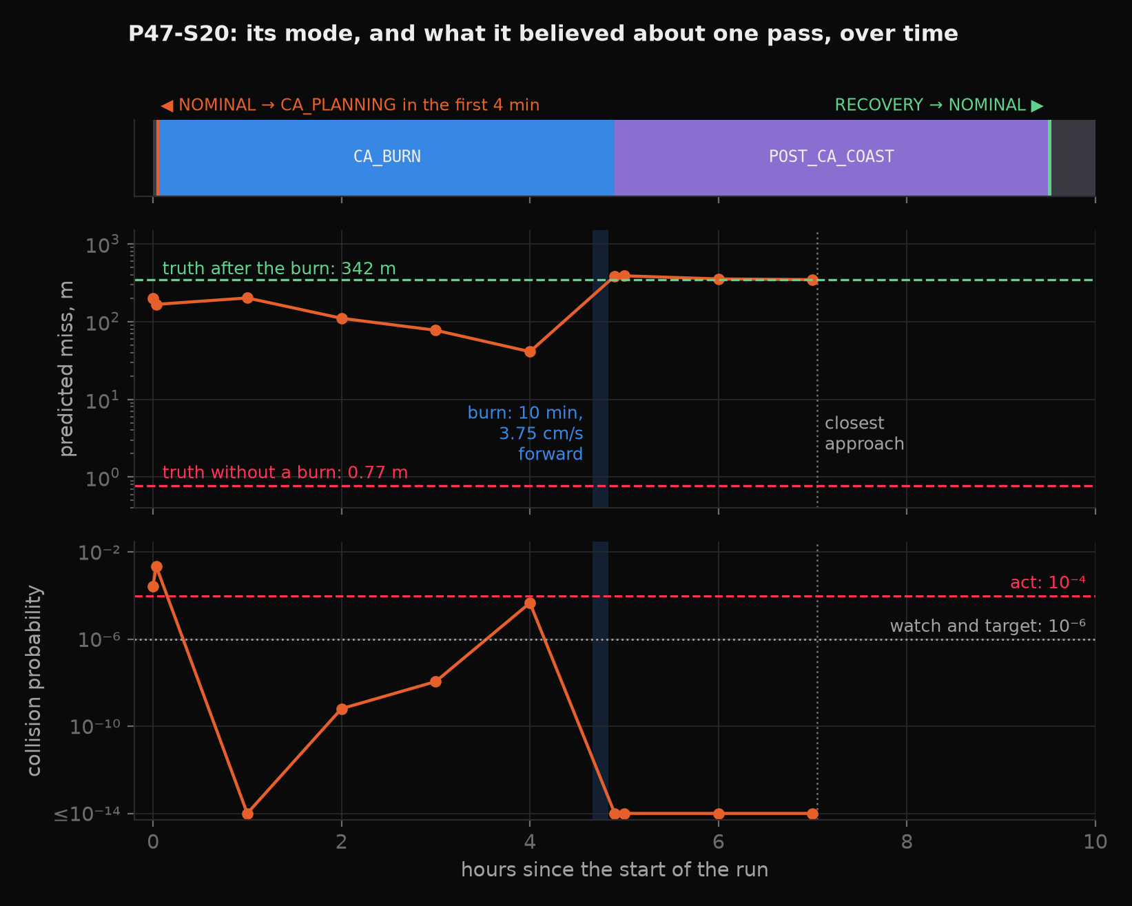
NOMINAL → CA_PLANNING: the first screening puts the pass at 200 m with a probability above 10⁻⁴. CA_PLANNING → CA_BURN two minutes later, with the burn queued for T+4 h 40 min. While it waits, the filter sharpens the prediction: 200, 110, 77, then 41 m. The burn fires for ten minutes, forward, 3.75 cm/s. POST_CA_COAST: the passes are reassessed from new measurements, 383, 352, then 344 m. The real miss is 342 m. RECOVERY begins only after the last pass of the series, at T+9 h 30 min, and the satellite is back to NOMINAL two minutes later.
The burn does not push the satellite sideways. Pushing forward raises the orbit, a higher orbit is slower, and over the 2.3 hours before the crossing the satellite falls behind its old schedule. The Clohessy–Wiltshire equations, which describe motion relative to a circular orbit, give the size of that effect for a short forward push :
For this burn ( = 3.75 cm/s, = 1.093 × 10⁻³ rad/s, and = 8,269 s from the middle of the burn) they predict the satellite ends up 132 m higher and 879 m behind. The simulated world, with a ten minute burn instead of an instant push and drag at the satellite’s hidden density, puts it 125 m higher and 843 m behind. The satellite reaches the crossing point about a tenth of a second late, and the object passes 342 m away.
6. Verification
Testing was layered, from single equations up to real data. Each layer had to pass before the next was worth running.
| Layer | What it checks | Scale |
|---|---|---|
| Unit tests | every equation against an analytic answer, every state machine transition on its own, the C++ core against the Python reference | more than 500 tests |
| End to end test | one planted collision course must go WATCH or PLANNING → BURN → COAST → RECOVERY → NOMINAL, with every pass below in truth and the slot recovered | one encounter, deterministic |
| Monte Carlo | the whole loop with random hidden errors | 96 satellites for 3 days; 40 encounters, flown with and without the filter |
| Scale | the full system on a Starlink-size shell | 1,600 satellites for 48 hours, 20 planted collision courses |
| Real data | screening against an independent operational service | the full public catalog against CelesTrak’s SOCRATES |
The last layer leaves the simulated world entirely. The fleet loads CelesTrak’s public orbit data for every tracked object and propagates it with SGP4, the standard model that data is published for. CelesTrak also runs SOCRATES, a collision screening service built on the commercial STK software, three times a day. For SOCRATES’s 25 closest Starlink conjunctions of the week, I took the exact orbit data SOCRATES used and screened each pair from scratch. The closest approach times agree within 0.48 ms and the miss distances within 0.50 m, which is the rounding in SOCRATES’s own reports.
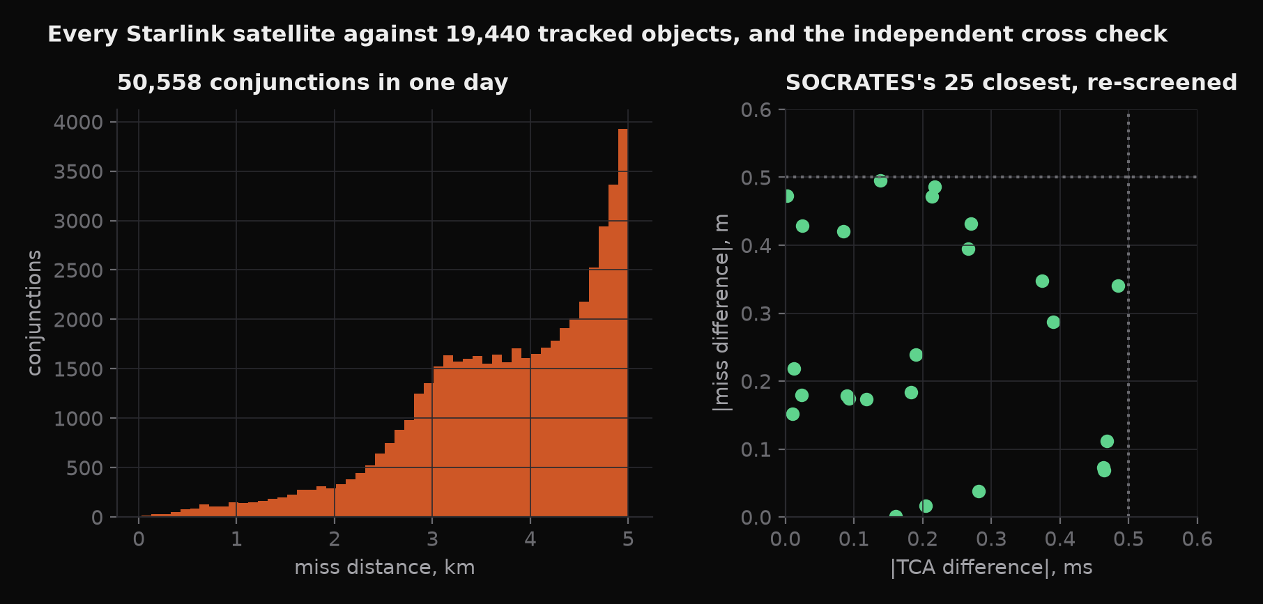
Left: all 11,151 Starlink satellites against all 19,440 tracked objects for one day, 50,558 passes under 5 km, about nine for each Starlink satellite. Right: SOCRATES’s 25 closest, screened again from SOCRATES’s own orbit data. Every one agrees within half a millisecond and half a metre.
Against the requirements from section 1:
| # | Requirement | Result | |
|---|---|---|---|
| 1 | No collisions, in truth | 0 of 40 Monte Carlo encounters, 0 of 12 in the 12 hour shell run, 0 of 20 in the 48 hour run | met |
| 2 | Every avoided encounter ends below | all 40 with the Kalman filter (37 of 40 without it) | met |
| 3 | Satellites stay in their slots | all 96 captured and held, typical orbit size error 27 m; the worst excursions reach 2.4 km before correction pulls them back | met |
| 4 | Back within 1 km of the slot after an avoidance | median 2.1 hours after closest approach | met |
| 5 | Propellant spent sparingly | avoidance 3.6 cm/s on average; station keeping 0.27 m/s over three days, including the initial capture, out of 2.1 km/s on board | met |
| 6 | No unsafe command flown | no SAFE entry in 40 encounters with the filter (one without it); no command refused in the 12 hour shell run | met |
| 7 | Faster than real time at full scale | 48 hours of the 1,600 satellite shell in 36 minutes, 80 times faster than real time | met |
7. Running at scale
Three changes took the system from 24 satellites to a full shell.
Choosing the phasing. A Starlink shell has 72 orbital planes of 22 satellites at 550 km and 53°. How the satellites in neighbouring planes are offset from one another is set by a single integer, the Walker phasing factor . With the obvious choice, , satellites in neighbouring planes pass 3.4 km apart every orbit, and the fleet spent its time checking itself: 4,743 passes in two hours. Trying every and keeping the one with the largest minimum distance gives , where no two satellites ever come within 71.5 km.
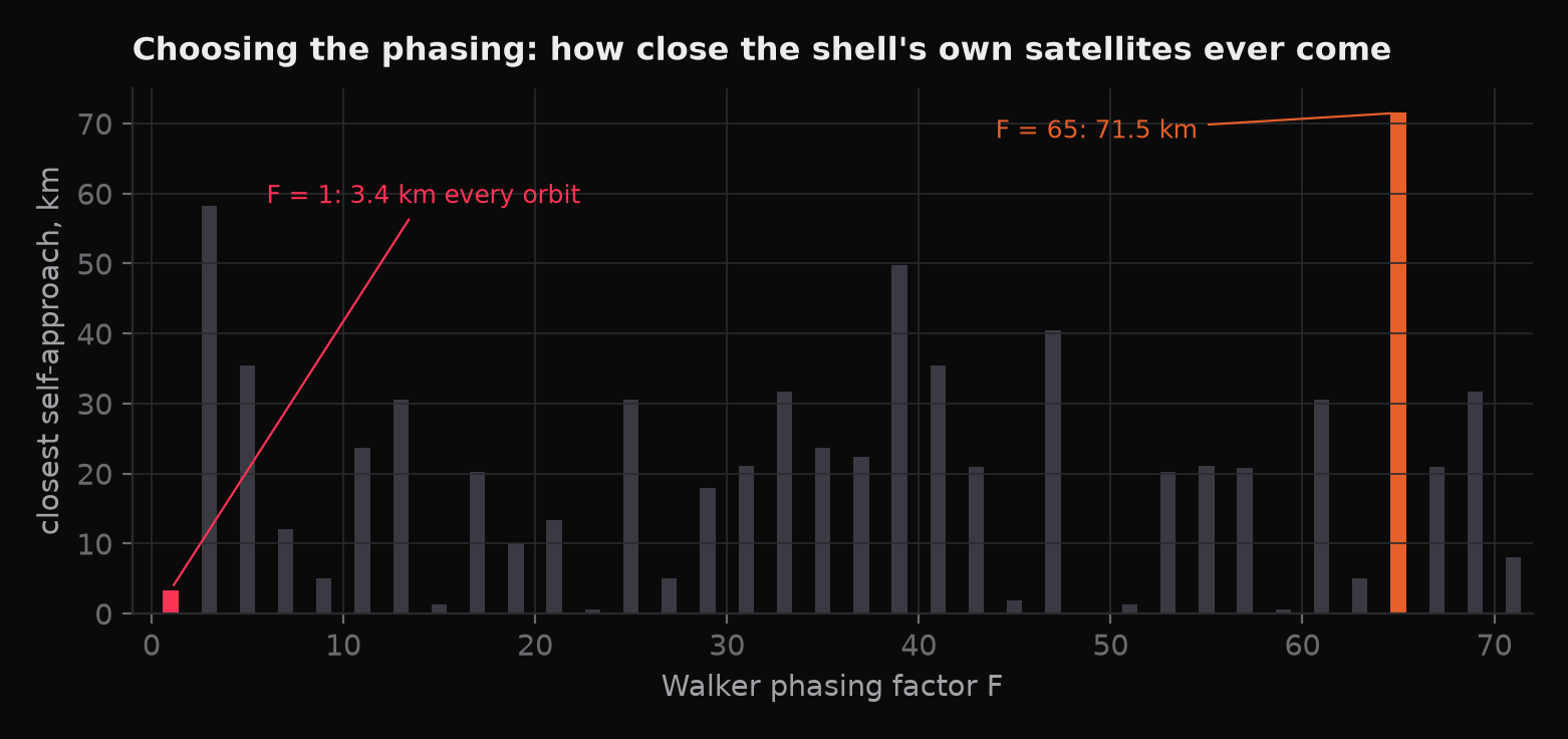
The closest any two satellites in the shell ever get, for every phasing factor. The obvious choice, , is one of the worst.
A screening grid that gives the exact answer. Checking every satellite against every object stops working at this size. Since each pass is resolved by straight line motion between samples, a pass that comes within the screening distance means the two objects were within
at one of the samples, where is the largest possible relative speed. So if space is divided into cubes of side , every pair that matters sits in the same cube or a neighbouring one, and only those pairs are checked. The tests confirm the grid finds exactly the passes that checking every pair finds.
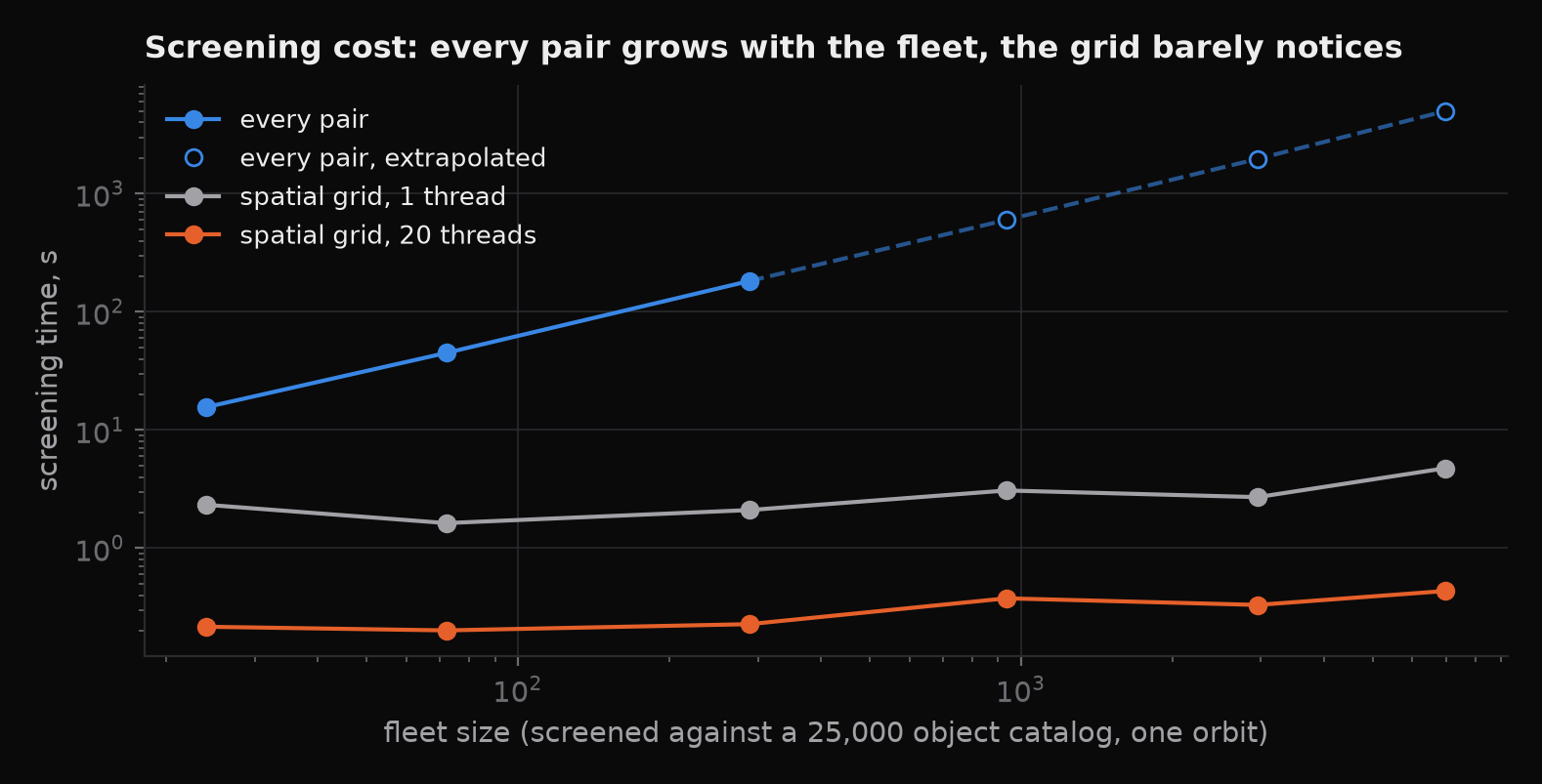
A Starlink-like shell checked against 25,000 tracked objects over one orbit. At 6,984 satellites, checking every pair would take about 84 minutes. The grid takes 0.44 s on 20 threads, because each object only looks at its own cube and the 26 around it, however large the fleet is.
A C++ core. Profiling one encounter showed that 79 of its 85 seconds were spent inside scipy’s integrator calling my Python force functions, 1.1 million times. I moved the integrator, the force models, and their derivatives to C++, called from Python through pybind11. I ported scipy’s own DOP853 integrator rather than switching to a different one, with the same coefficients and error control, compiled so its rounding matches numpy’s. That kept the Python version as a reference the C++ one could be checked against line for line. On the 40 test encounters both make exactly the same decisions.
| Python | C++ | speedup | |
|---|---|---|---|
| one fleet integration | 380 ms | 2.9 ms | 130× |
| one encounter, end to end | 65 s | 4.7 s | 14× |
| Monte Carlo, 96 + 40 runs on 20 cores | 607 s | 56 s | 10.8× |
| full test suite | 9 min 16 s | 1 min 23 s | 6.7× |
8. Limits and next steps
- The thresholds are for the study. , , the 2 km slot box, and the 3 hour deadline were chosen to exercise the design, not taken from an operator.
- The planner searches a grid. Ninety candidates in six fixed directions find a good burn, not the best one. A continuous optimizer over direction and timing is the next step for the planner.
- One satellite maneuvers per encounter. When two of the fleet’s own satellites meet, only one is allowed to move. Coordinating both, or many in a crowded region, is the distributed extension in the design specification.
- Measurements are simulated. Navigation assumes GNSS-quality positions (5 m) for our satellites and 10 m tracking for everything else. The real catalog test covers screening, not navigation.
- Momentum is not dumped. Each turn borrows reaction wheel momentum and returns it. Long missions would need magnetorquers to unload the wheels.
Related projects
Nonlinear MPC for Autonomous Racing
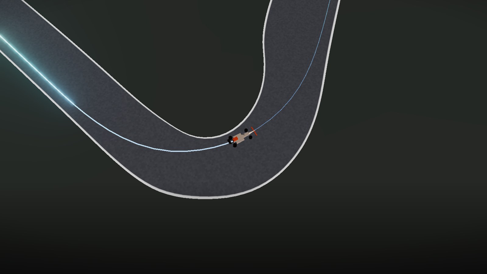
A controller for a full-scale Dallara AV-24 in the Indy Autonomous Challenge, built on two timescales: a minimum-time lap solved offline with a double-track Pacejka tyre model, and a progress-maximizing MPC that drives it at 100 Hz. My part is the offline layer, which produces the racing lines the online controller follows. Validated in software in the loop, in simulation at Laguna Seca (117.6 s, 25% faster than the baseline controller), and on the physical car.
Classical ML from Scratch
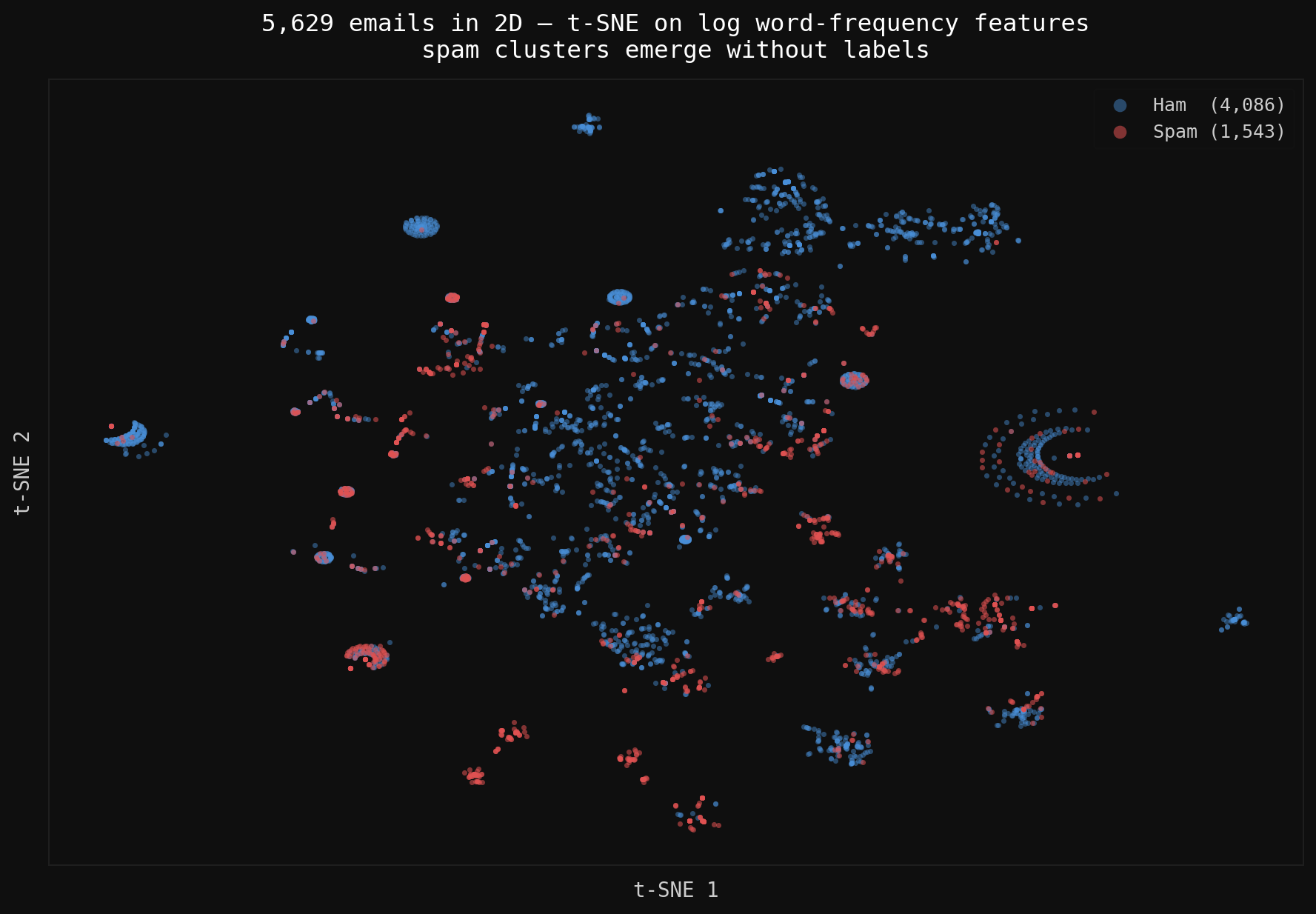
Two learning paradigms built from NumPy up: tree-based spam classification (decision tree, Random Forest, AdaBoost) and SVD/ALS matrix factorization for movie recommendations. No frameworks; matched scikit-learn on both.
Filters & Frequencies: Edges, Hybrid Images, and Blending
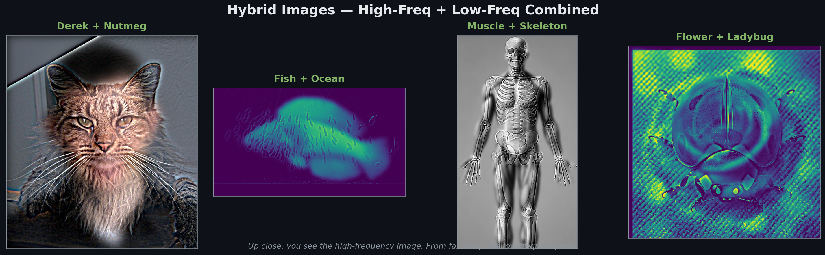
Working in the frequency domain to extract edges, create hybrid images that change meaning with viewing distance, and blend images seamlessly via Laplacian pyramids. Ends with the famous 'oraple.'