Neural Radiance Fields (NeRF)
Training an MLP to represent a 3D scene as a continuous function from (x, y, z, θ, φ) to (RGB, density). Volume rendering turns the field back into images; the field itself is the 3D model.
A NeRF is a neural network whose weights are the 3D scene. Given a 5D input (3D point location + viewing direction), the MLP outputs the RGB color and volume density at that point. Volumetric rendering integrates along camera rays to produce an image. Train on a few dozen photos of the object from known viewpoints, and the network learns a continuous 3D field you can then render from any new angle.
Part 1: Fitting a Neural Field to a 2D Image
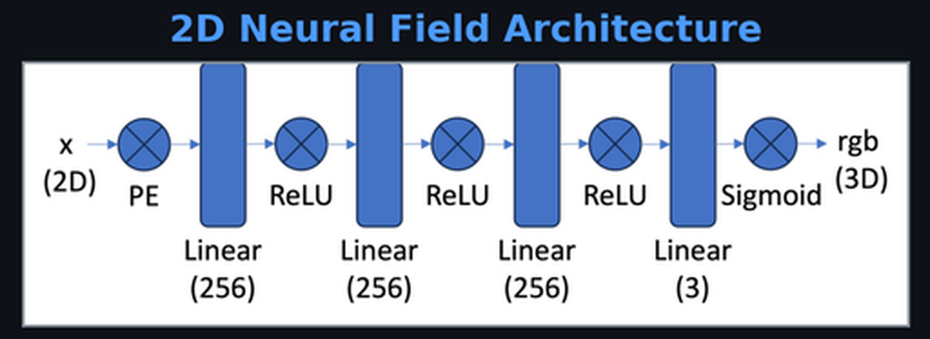
Before 3D, warm up with 2D. Train an MLP to map (x, y) pixel coordinates → RGB color. With no positional encoding, the MLP produces a blurry low-frequency approximation of the image; neural networks naturally learn smooth functions and can’t express sharp edges with raw coordinates as input.
Positional encoding fixes this. Each coordinate is expanded into sin/cos pairs at frequency octaves:
Applied to both x and y, the 2D input expands to 40 features. This gives the network a rich Fourier basis; instead of learning high-frequency functions from scratch (which smooth MLPs resist), it just weights the provided sinusoids. PSNR jumps from ~12 dB (unrecognizable) to ~28 dB (nearly indistinguishable from ground truth).
Part 2: 3D NeRF on Lego
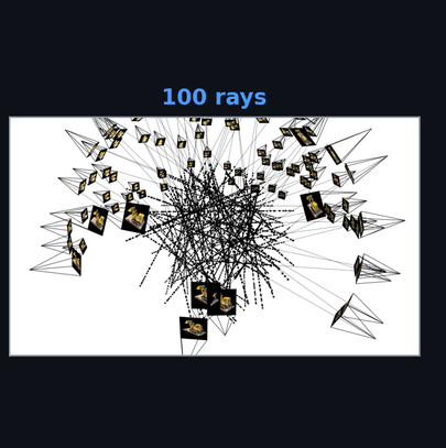
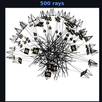
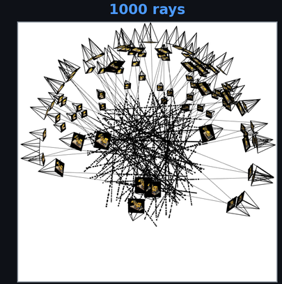
Ray sampling is the central bridge between the network and the image. For each target pixel, a ray is cast from camera origin through the pixel. points are sampled along the ray; the NeRF is queried at each for color and density . These are composited via the volume rendering integral:
is transmittance, the probability the ray reaches without being absorbed. The integral weights each point’s color by how much of the ray’s “budget” is deposited there. In practice, the continuous integral is replaced by the discrete approximation used during training:
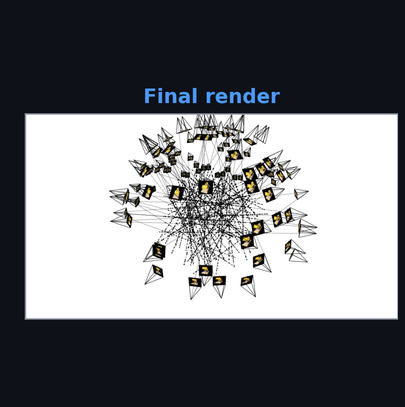
The visualization above shows rays sampled in increasing count (100 → 1000 → final full render). Each ray contributes one pixel. 100k+ rays per image × 100 training images = ~10M training examples.
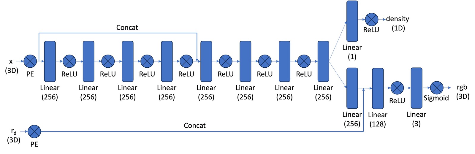
The architecture, an 8-layer MLP with skip connection, is remarkably simple for what it accomplishes. The position is expanded via positional encoding (, giving 60 features) and passed through 8 Linear(256)/ReLU layers with a skip connection at layer 5. Density branches off the 8th layer. The viewing direction is positional-encoded separately (, 24 features) and concatenated before the color head: Linear(256) → Linear(128) → Linear(3)/Sigmoid → RGB.
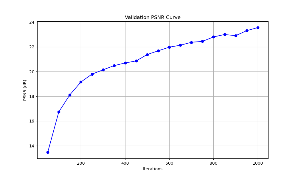
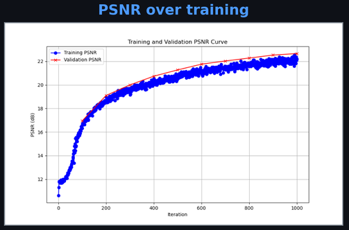
PSNR reaches ~23.5 dB after 1000 iterations on the Lego scene.
Novel View Synthesis
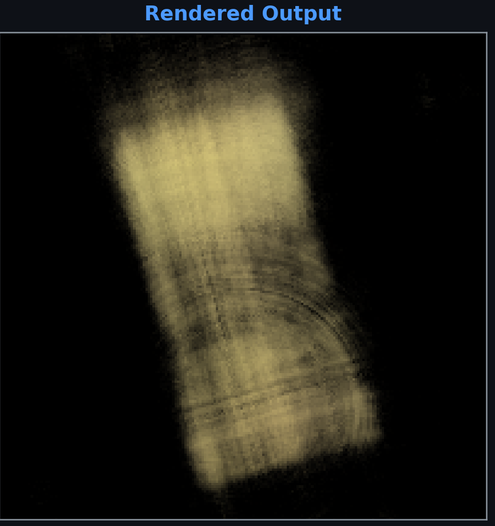
The payoff: render the scene from viewpoints no camera ever saw. Once the NeRF is trained, any new (camera origin, viewing direction) combination can be rendered by casting rays and querying the MLP. The GIFs above show full 360° turntable renders synthesized from the learned field; the model has captured not just surface appearance but the full volumetric structure.
Depth maps fall out for free. The volume density σ tells us where surfaces are along each ray; integrating ray distance weighted by density gives expected surface depth. No explicit depth supervision during training; the geometry emerges implicitly from the multi-view constraint.
The profound part: a small MLP (~1M parameters) compresses 100 photos of a scene into a single continuous 3D function. The representation is implicit: no mesh, no voxels, no point cloud. Just weights in a neural network, and a rendering equation that makes those weights correspond to a visual world.
Related projects
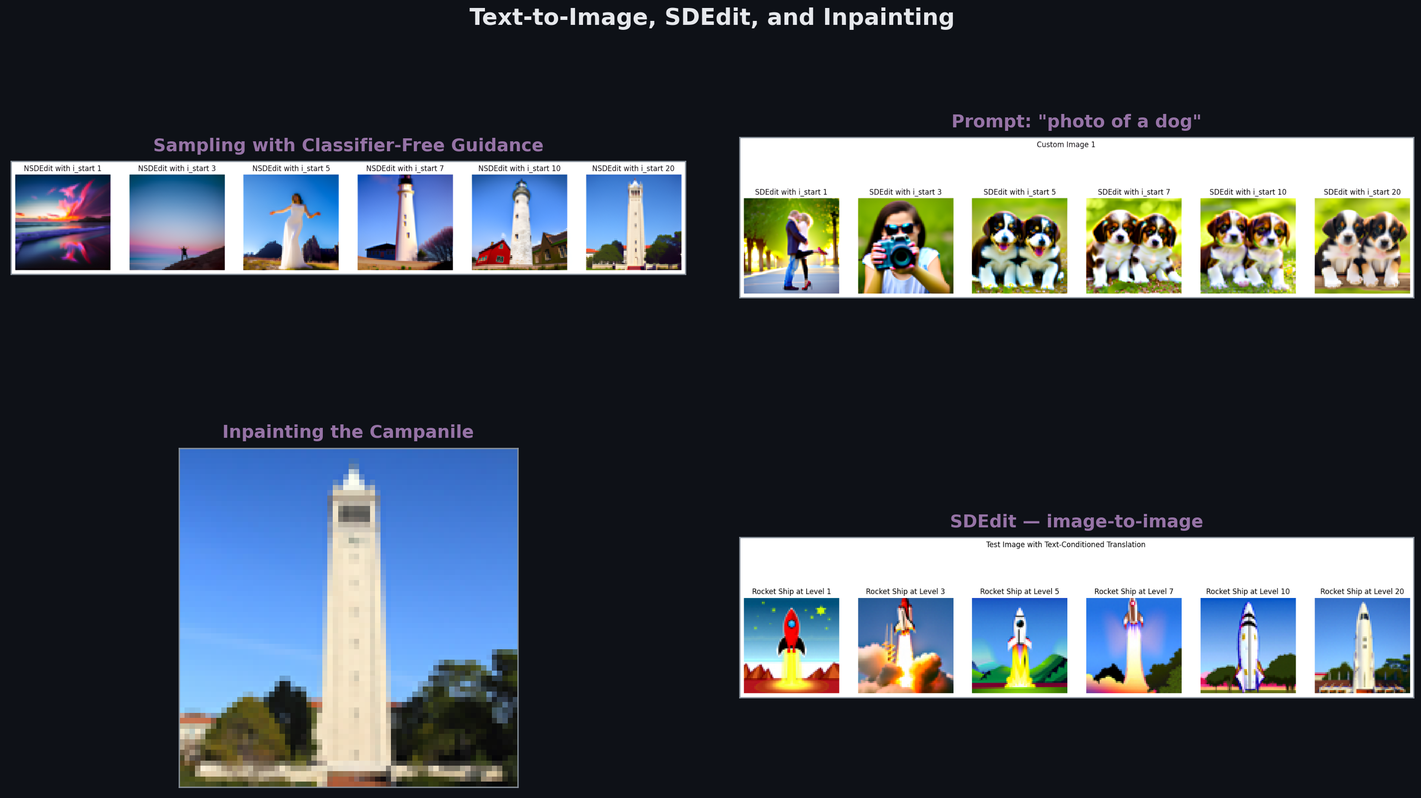
Fun With Diffusion Models
Sampling from DeepFloyd IF (CFG, SDEdit, inpainting, visual anagrams), then training a time- and class-conditioned U-Net from scratch on MNIST to learn the diffusion process end-to-end.
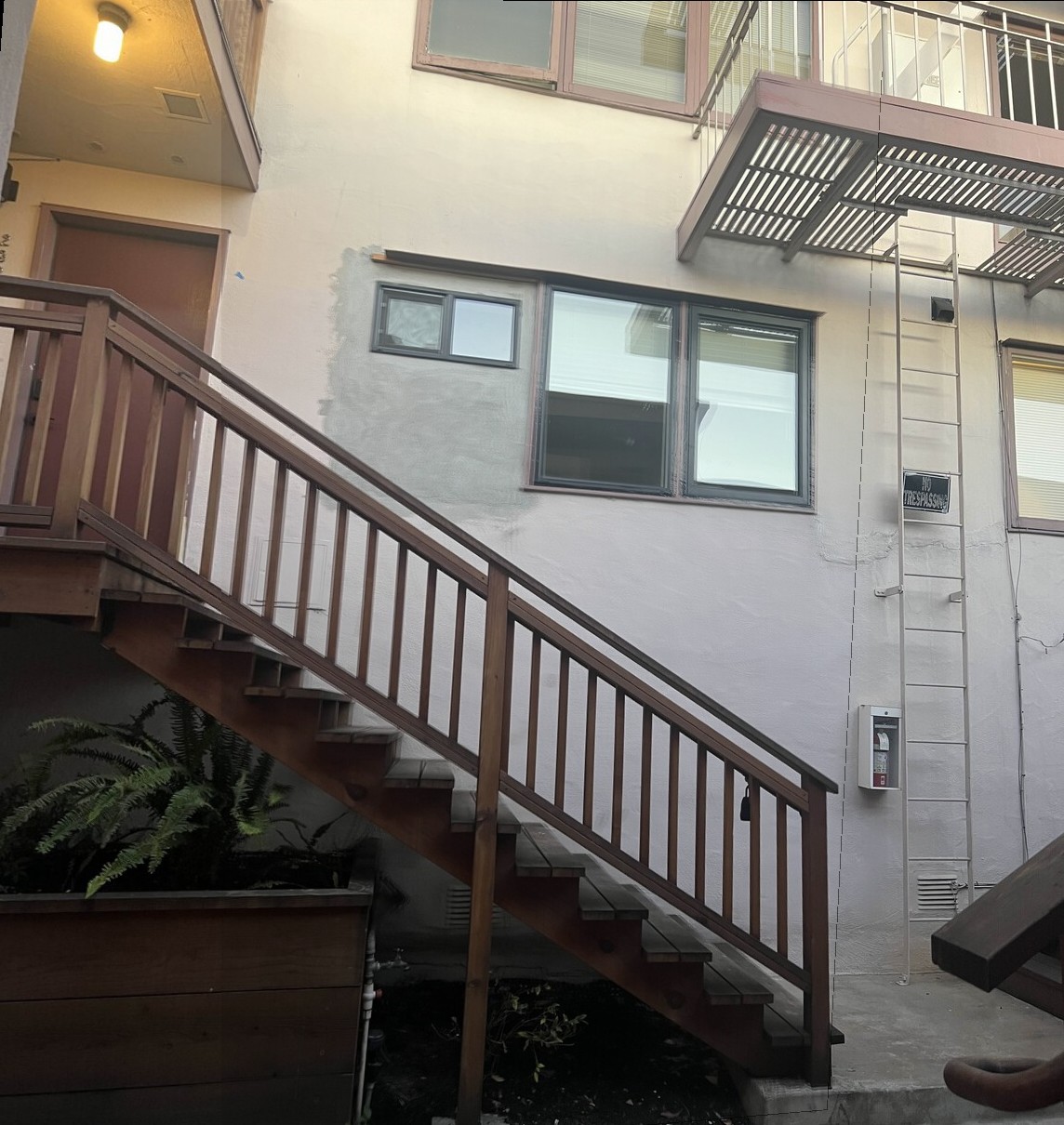
Auto-Stitching Photo Mosaics
Building a panorama pipeline from scratch: Harris corner detection, Adaptive Non-Maximal Suppression, feature matching, RANSAC for homography estimation, and Laplacian-pyramid blending.
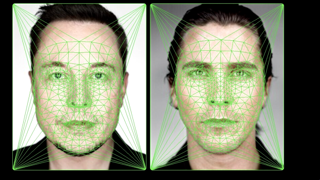
Face Morphing with Delaunay Triangulation
Smooth warping between two faces via point correspondences, Delaunay triangulation, and affine warps per triangle. Plus: population mean faces and caricature generation by extrapolation.